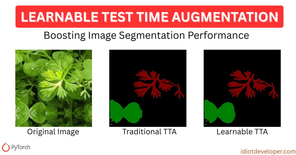
Test Time Augmentation (TTA) is a simple yet powerful technique to improve image segmentation results by applying multiple transformations to an input image during inference and combining the outputs. When paired with models like U-Net, it often boosts performance without retraining.
But what if we could go one step further and learn how to optimally combine those augmented predictions? That’s the promise of Learnable Test Time Augmentation, and in this article, we’ll break down its core logic, explain the complete PyTorch implementation, and show how it outperforms traditional methods.
What is Test Time Augmentation?
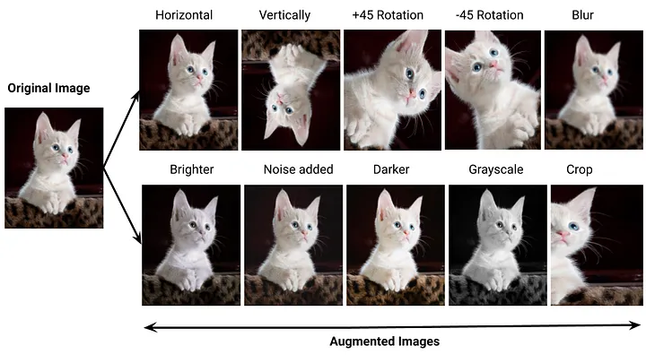
It is a commonly used technique where multiple augmented versions of an image are passed through a trained model, and the outputs are fused to produce a more robust prediction.
TTA is used during inference to make predictions more robust by:
- Generating multiple augmented versions of the input image (e.g., flips, rotations).
- Passing each variant through the model.
- Reversing the augmentations on the predictions.
- Averaging all predictions to form the final output.
It’s commonly used in image segmentation, classification, and detection pipelines, especially when deploying models in critical environments.
READ MORE: Test Time Augmentation (TTA) for Segmentation in PyTorch
Limitations of Traditional TTA
Despite its utility, traditional TTA has a few drawbacks:
- Uniform Averaging: It treats all augmented predictions equally—even if some augmentations hurt performance.
- No Adaptability: It cannot learn from the data.
- Prediction Noise: In some augmentations, model performance may degrade due to semantic inconsistency.
Hence, there’s room to improve by making the fusion process smarter.
Learnable TTA
Learnable TTA adds a lightweight neural module that learns how to best combine predictions from multiple augmentations.
Key Features:
- Uses a learnable weight for each augmented prediction.
- Applies softmax to normalize weights.
- Combines predictions using a weighted sum.
- Trained using a small validation set with CrossEntropy loss.
This intelligent fusion results in more accurate segmentation predictions.
Code Repo: Multiclass Segmentation in PyTorch
Code Implementation
Let’s break the code down step by step.
Imports
We import essential libraries for data loading, model building, evaluation, and augmentation:
import os
import time
import numpy as np
from glob import glob
import cv2
from tqdm import tqdm
import torch
import torch.nn as nn
import torch.nn.functional as F
from model import build_unet
from utils import create_dir, seeding
from train import load_data
from sklearn.metrics import f1_score, jaccard_score
Configure CUDA
Set the visible GPU if available:
os.environ["CUDA_VISIBLE_DEVICES"] = "0" if torch.cuda.is_available() else ""
device = torch.device("cuda" if torch.cuda.is_available() else "cpu")
Image Processing
Handles:
- Resizing and normalizing input images
- Converting RGB masks to class indices and back
class ImageProcessor:
    def __init__(self, size, colormap):
        self.size = size
        self.colormap = colormap
        self.num_classes = len(colormap)

    def process_image(self, image_path):
        image = cv2.imread(image_path, cv2.IMREAD_COLOR)
        image = cv2.resize(image, self.size)
        image = np.transpose(image, (2, 0, 1)) / 255.0
        return torch.from_numpy(image).float().to(device)

    def process_mask(self, mask_path):
        mask = cv2.imread(mask_path, cv2.IMREAD_COLOR)
        mask = cv2.resize(mask, self.size)
        target = np.zeros((mask.shape[0], mask.shape[1]), dtype=np.int64)
        for class_id, color in enumerate(self.colormap):
            target[np.all(mask == color, axis=-1)] = class_id
        return torch.from_numpy(target).long().to(device)

    def mask_to_rgb(self, mask):
        height, width = mask.shape
        rgb_mask = np.zeros((height, width, 3), dtype=np.uint8)
        for class_id, rgb in enumerate(self.colormap):
            rgb_mask[mask == class_id] = rgb
        return rgb_mask
Apply Augmentations
This function applies test-time augmentations:
- Original
- Horizontal flip
- Vertical flip
- Horizontal + Vertical flip
It then collects predictions for each version.
def apply_augmentations(model, image_tensor):
    model.eval()
    predictions = []

    with torch.no_grad():
        # Original
        pred_orig = torch.softmax(model(image_tensor), dim=1)
        predictions.append(pred_orig)

        # Horizontal flip
        img_hflip = torch.flip(image_tensor, dims=[3])
        pred_hflip = torch.flip(torch.softmax(model(img_hflip), dim=1), dims=[3])
        predictions.append(pred_hflip)

        # Vertical flip
        img_vflip = torch.flip(image_tensor, dims=[2])
        pred_vflip = torch.flip(torch.softmax(model(img_vflip), dim=1), dims=[2])
        predictions.append(pred_vflip)

        # Horizontal + Vertical flip
        img_hvflip = torch.flip(image_tensor, dims=[2, 3])
        pred_hvflip = torch.flip(torch.softmax(model(img_hvflip), dim=1), dims=[2, 3])
        predictions.append(pred_hvflip)

    return predictions
LearnableTTA Class
LearnableTTA is the core module that replaces simple averaging. It is a small neural network that learns to combine multiple predictions. Instead of simply averaging, it assigns learnable weights to each augmented version.
class LearnableTTA(nn.Module):
    def __init__(self, num_transforms=4):
        super().__init__()
        self.num_transforms = num_transforms
        self.weights = nn.Parameter(torch.ones(num_transforms))

    def forward(self, preds):
     # Apply softmax to get normalized weights for fusion
        weights = torch.softmax(self.weights, dim=0).to(preds[0].device)
        stacked = torch.stack(preds, dim=0)
        # Weighted sum of predictions
        weighted_preds = (weights.view(-1, 1, 1, 1, 1) * stacked).sum(dim=0)
        return weighted_preds
Training: Learnable TTA
This function trains the Learnable TTA module using a small validation set. We apply augmentations, get predictions, and let the TTA module learn how to best combine them.
def train_learnable_tta(model, tta_module, val_x, val_y, processor, epochs=5):
    model.eval()
    tta_module.train()
    optimizer = torch.optim.Adam(tta_module.parameters(), lr=0.01)
    criterion = nn.CrossEntropyLoss()

    # Pre-process all validation data
    val_data = []
    for x, y in zip(val_x, val_y):
        image = processor.process_image(x)
        mask = processor.process_mask(y)
        val_data.append((image.unsqueeze(0), mask.unsqueeze(0)))

    for epoch in range(epochs):
        total_loss = 0
        for image, target in tqdm(val_data, desc=f"Epoch {epoch+1}"):
            preds = apply_augmentations(model, image)
            final_pred = tta_module(preds)

            loss = criterion(final_pred, target)
            optimizer.zero_grad()
            loss.backward()
            optimizer.step()
            total_loss += loss.item()

        print(f"Epoch {epoch+1} Loss: {total_loss/len(val_data):.4f}")
Evaluation
This function evaluates the model with the trained Learnable TTA module. It saves visualization results, computes F1 and IoU, and logs performance metrics.
def evaluate(model, tta_module, save_path, test_x, test_y, processor, classes):
    time_taken = []
    scores = []

    create_dir(f"{save_path}/mask")
    create_dir(f"{save_path}/joint")

    for x, y in tqdm(zip(test_x, test_y), total=len(test_x)):
        name = os.path.splitext(os.path.basename(y))[0]
        image = processor.process_image(x)
        mask = processor.process_mask(y)

        # Save original images for visualization
        save_img = (image.cpu().numpy().transpose(1, 2, 0) * 255).astype(np.uint8)
        save_mask = processor.mask_to_rgb(mask.cpu().numpy())

        with torch.no_grad():
            start_time = time.time()
            preds = apply_augmentations(model, image.unsqueeze(0))
            final_pred = tta_module(preds)
            y_pred = torch.argmax(final_pred, dim=1).squeeze(0).cpu().numpy()
            time_taken.append(time.time() - start_time)

        # Save results
        line = np.ones((processor.size[1], 10, 3)) * 255
        pred_rgb = processor.mask_to_rgb(y_pred)
        cat_images = np.concatenate([save_img, line, save_mask, line, pred_rgb], axis=1)
        cv2.imwrite(f"{save_path}/joint/{name}.jpg", cat_images)
        cv2.imwrite(f"{save_path}/mask/{name}.jpg", pred_rgb)

        # Calculate metrics
        y_true = mask.cpu().numpy().flatten()
        y_pred = y_pred.flatten()

        f1_value = f1_score(y_true, y_pred, labels=range(processor.num_classes),
                           average=None, zero_division=0)
        jac_value = jaccard_score(y_true, y_pred, labels=range(processor.num_classes),
                              average=None, zero_division=0)
        scores.append([f1_value, jac_value])

    # Calculate and print final metrics
    scores = np.mean(np.array(scores), axis=0)
    print("Class           F1         IoU")
    print("-"*35)

    with open(f"files/scores_learnable_tta.csv", "w") as f:
        f.write("Class,F1,Jaccard\n")
        for i, class_name in enumerate(classes):
            print(f"{class_name:15s}: {scores[0, i]:.5f} - {scores[1, i]:.5f}")
            f.write(f"{class_name},{scores[0, i]:.5f},{scores[1, i]:.5f}\n")

        mean_f1 = np.mean(scores[0])
        mean_jac = np.mean(scores[1])
        print("-"*35)
        print(f"{'Mean':15s}: {mean_f1:.5f} - {mean_jac:.5f}")
        f.write(f"Mean,{mean_f1:.5f},{mean_jac:.5f}\n")

    fps = 1 / np.mean(time_taken)
    print(f"Mean FPS: {fps:.2f}")
    return fps
Execution of Learnable TTA
Finally, in the main block:
- Set configuration: paths, image size, colormap.
- Load trained U-Net model.
- Prepare validation and test sets.
- Train LearnableTTA for a few epochs.
- Evaluate performance.
if __name__ == "__main__":
    seeding(42)

    # Configuration
    config = {
        "image_size": (256, 256),
        "dataset_path": "./Weeds-Dataset/weed_augmented",
        "colormap": [[0, 0, 0], [0, 0, 128], [0, 128, 0]],
        "classes": ["background", "Weed-1", "Weed-2"],
        "checkpoint_path": "files/checkpoint.pth",
        "save_path": "results_learnable_tta",
        "tta_epochs": 5
    }

    # Initialize components
    processor = ImageProcessor(config["image_size"], config["colormap"])
    model = build_unet(num_classes=processor.num_classes).to(device)
    model.load_state_dict(torch.load(config["checkpoint_path"], map_location=device)["model_state_dict"])
    model.eval()

    # Load data
    (train_x, train_y), (valid_x, valid_y), (test_x, test_y) = load_data(config["dataset_path"])
    valid_x, valid_y = valid_x[:100], valid_y[:100]  # Use subset for TTA training

    # Create and train the Learnable TTA module
    tta_module = LearnableTTA().to(device)
    train_learnable_tta(model, tta_module, valid_x, valid_y, processor, epochs=config["tta_epochs"])

    # Finally, evaluate on the test set using Learnable TTA
    evaluate(model, tta_module, config["save_path"], test_x, test_y, processor, config["classes"])
Performance Comparison
| Method | F1 Score | mIoU |
| No TTA (Baseline) | 0.44360 | 0.36687 |
| Traditional TTA | 0.52263 | 0.47479 |
| Learnable TTA | 0.67362 | 0.63462 |
Result: Learnable TTA improves mIoU by ~15% over traditional averaging.
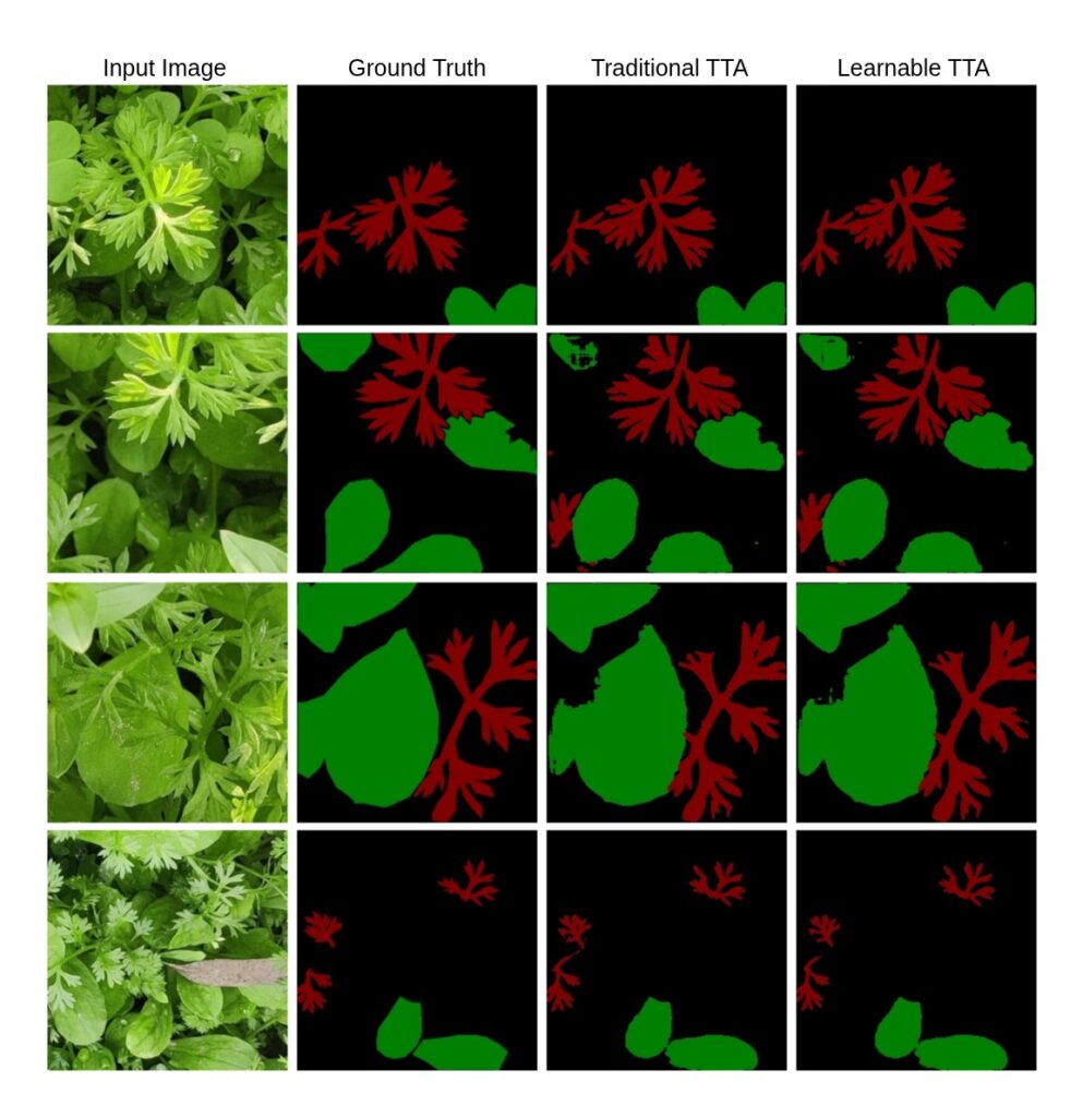
Learnable TTA not only enhances accuracy quantitatively (as shown in earlier tables) but also delivers visibly better results, particularly in challenging regions with complex textures or shapes. This makes it a highly effective plug-in module for image segmentation models like UNet.
Where This Shines
Learnable TTA is especially powerful for:
- Medical Imaging: Where misclassification can be critical.
- Agriculture: For pixel-wise plant and weed detection.
- Autonomous Systems: Where reliable predictions drive safety.
Limitations and Considerations
- Needs a small validation set for learning weights.
- Overfitting is possible on limited validation data.
- Augmentation quality affects the learned weights.
Still, these are minor compared to the performance gain.
Conclusion & Resources
If you’re already using Test Time Augmentation in your U-Net image segmentation workflows, switching to a Learnable TTA module is a low-cost, high-reward improvement.
Video Tutorial: Watch on YouTube
Code Repo: Multiclass Segmentation in PyTorch
Dataset: Multiclass Weeds Dataset
What Next?
Explore further enhancements:
- Add more augmentations (rotate, scale)
- Try with other segmentation models (DeepLabV3+, SegFormer)
- Combine Learnable TTA with Uncertainty Estimation
Want more posts like this? Follow me for practical tutorials on PyTorch, Image Segmentation, and real-world ML.
Stay tuned
