In high-stakes fields like medical imaging, autonomous driving, and remote sensing, a wrong prediction made with high confidence can be catastrophic. That’s where Uncertainty Estimation steps in—empowering your model to express doubt. And with techniques like Monte Carlo Dropout, you can transform any deterministic deep network into a model that not only predicts—but knows when it’s uncertain.
In this tutorial, we’ll explore Uncertainty Estimation in Multiclass Image Segmentation using the widely-adopted UNet architecture combined with Monte Carlo Dropout, all implemented in PyTorch. Inspired by Bayesian deep learning, this method enables your model to generate pixel-wise confidence maps, offering much more than just the final prediction.
You’ll learn two practical approaches:
- Injecting dropout layers into a pre-trained model at inference time
- Training the model with dropout layers from scratch
By the end, you’ll be able to generate and interpret uncertainty heatmaps, identify where your model might fail, and take the first step toward making your AI more trustworthy and transparent.
Let’s break it down.
Code: Multiclass Segmentation in PyTorch
What is Uncertainty Estimation?
In simple terms, Uncertainty Estimation helps us measure how confident a model is about its predictions. Unlike traditional deep learning models that output a single deterministic prediction, uncertainty-aware models return a distribution of possible outcomes, helping identify areas where the model is unsure.
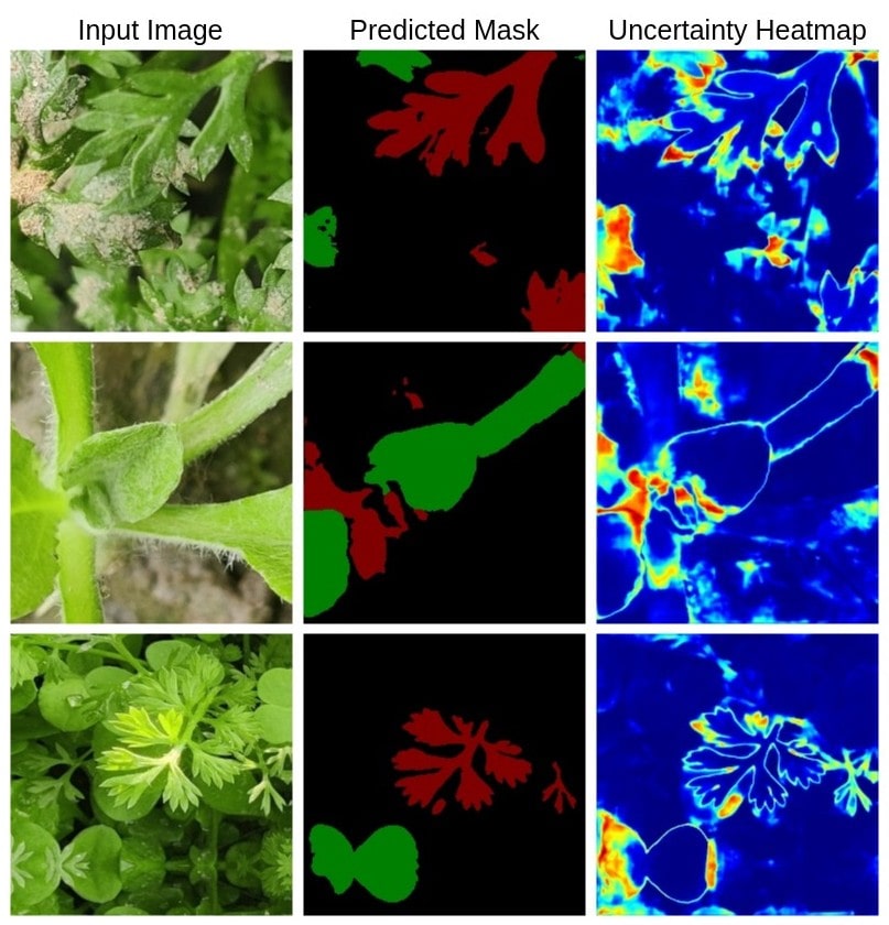
In segmentation, we can visualize uncertainty as heatmaps—areas where the model has low confidence are highlighted, allowing for targeted review or fallback strategies.
ALSO READ: GradCAM Heatmaps for Segmentation with UNet in PyTorch
Why Uncertainty Estimation Matters?
Imagine a medical image segmentation model misclassifying a tumor boundary with high confidence. Without uncertainty feedback, such a mistake may go unnoticed. However, with Monte Carlo Dropout-based Uncertainty Estimation, the same model can signal, “I’m unsure about this region”, prompting a radiologist to inspect more closely.
In practice, uncertainty maps help in:
- Error Detection – Flagging unreliable predictions
- Active Learning – Selecting informative samples for re-labeling
- Model Explainability – Understanding the limits of your model
- Risk-aware Decision Making – Particularly in critical fields like healthcare or autonomous navigation
Uncertainty isn’t just academic—it’s a gateway to safer, smarter, and more robust AI systems.
Approaches for Uncertainty Estimation
In this article, we focus on Monte Carlo Dropout, a scalable and practical way to approximate Bayesian inference in deep neural networks. Unlike traditional dropout (used only during training), MC Dropout is applied during inference to simulate an ensemble of models by performing multiple stochastic forward passes.
We implement two core approaches using a UNet model in PyTorch:
Approach 1: Inject Dropout After Training
We take a pre-trained UNet and dynamically insert Dropout2D layers into the decoder (typically after ReLU activations). This allows us to run Monte Carlo inference without retraining the model. It’s fast, flexible, and especially useful when you don’t want to alter your training pipeline.
Approach 2: Train the Model with Dropout
Here, we embed dropout layers into the model architecture during training. This allows the model to learn robustness against dropped neurons from the beginning. At inference time, we keep dropout active and perform multiple stochastic passes to estimate uncertainty.
Both approaches help generate predictive mean masks (final predictions) and uncertainty maps (regions of ambiguity), but serve different use-cases depending on your workflow.
Real-World Applications of Uncertainty Estimation
Uncertainty estimation isn’t just a research buzzword — it’s a critical safety layer in real-world AI systems. Here’s how it’s transforming applications across domains:
- Medical Imaging: In tasks like tumor boundary segmentation or organ detection, uncertainty maps help radiologists identify ambiguous regions, reduce false positives, and make more informed decisions. It acts like a second opinion — powered by AI.
- Precision Agriculture: In weed and crop segmentation, high uncertainty often arises at overlapping or occluded leaves. Highlighting these regions can assist in selective herbicide spraying or manual verification.
- Autonomous Driving: Uncertainty maps help flag unseen or out-of-distribution objects, such as construction barriers or pedestrians in unusual poses. This enhances safety by alerting fallback systems.
- Active Learning: Models can suggest which uncertain images should be labeled next, reducing labeling effort while improving dataset quality — perfect for domain-specific segmentation problems.
- Model Debugging and Calibration: When a model fails silently, uncertainty estimation helps you visualize failure regions. This supports better diagnostics, debugging, and iterative improvement of your segmentation pipeline.
Code Walkthrough: Uncertainty Estimation via Post-Training Dropout Injection
For this tutorial, we focus on the more flexible and non-intrusive strategy — injecting Dropout layers into a pre-trained UNet decoder. This lets you estimate epistemic uncertainty without the need to retrain the model from scratch.
Let’s break down the core components of the implementation:
Injecting Dropout After Training
Instead of modifying your network architecture manually, we dynamically insert nn.Dropout2d layers after every ReLU activation in the decoder stages of UNet:
def add_dropout_to_decoder(model, p=0.5):
    for decoder_name in ["d1", "d2", "d3", "d4"]:
        decoder_block = getattr(model, decoder_name)
        conv_block = decoder_block.conv.conv

        new_layers = []
        for layer in conv_block:
            new_layers.append(layer)
            if isinstance(layer, nn.ReLU):
                new_layers.append(nn.Dropout2d(p))

        decoder_block.conv.conv = nn.Sequential(*new_layers)
This function ensures that during inference, each forward pass randomly deactivates neurons — giving us different outputs for the same input image. These variations are key to estimating model uncertainty.
Arguments:
- model: The UNet model (or similar) whose decoder blocks you want to modify.
- p: Probability of dropout — the chance of each neuron being zeroed out. Default is 0.5.
It loops through decoder stages (d1 to d4) and inserts a Dropout2d layer after every ReLU in the conv_block. This is useful for test-time stochasticity to estimate uncertainty.
Monte Carlo Dropout Inference
The core idea of Monte Carlo Dropout is to perform T stochastic forward passes and observe the distribution of outputs. Here’s how we do it:
def mc_dropout_inference(model, image_tensor, T=20):
    model.train()  # Keep dropout layers active during inference
    preds = []

    with torch.no_grad():
        for _ in range(T):
            output = model(image_tensor)
            probs = torch.softmax(output, dim=1)
            preds.append(probs.cpu().numpy())

    preds = np.stack(preds, axis=0)  # [T, C, H, W]
    mean_prob = np.mean(preds, axis=0)[0]  # Final prediction
    std_prob = np.std(preds, axis=0)[0]    # Uncertainty map

    return mean_prob, std_prob
This is the core function that performs Monte Carlo Dropout Inference.
Arguments:
- model: The dropout-injected UNet model.
- image_tensor: The input image tensor of shape [1, C, H, W], normalized and moved to device.
- T: Number of stochastic forward passes to perform (default: 20). More passes improve the estimate at the cost of computation.
Returns:
- mean_prob: Mean of softmax outputs over T passes; final class probability map of shape [C, H, W].
- std_prob: Standard deviation of predictions over T passes; represents uncertainty in model prediction, also shape [C, H, W].
The model is kept in train() mode to activate dropout during inference. For each pass, the function performs a forward pass, computes softmax, and stores the result. It returns the mean prediction and standard deviation for uncertainty.
Generating the Uncertainty Heatmap
We visualize the results by combining:
- Original image
- Segmentation prediction (colored)
- Uncertainty heatmap (color-mapped using COLORMAP_JET)
def run_uncertainty(model, test_x, size, colormap, save_dir, T=20):
    os.makedirs(save_dir, exist_ok=True)

    for path in tqdm(test_x, total=len(test_x)):
        name = path.split("/")[-1].split(".")[0]

        image = cv2.imread(path, cv2.IMREAD_COLOR)
        image = cv2.resize(image, size)
        orig_image = image.copy()

        input_tensor = np.transpose(image, (2, 0, 1)) / 255.0  # [C, H, W]
        input_tensor = np.expand_dims(input_tensor, axis=0).astype(np.float32)
        input_tensor = torch.from_numpy(input_tensor).to(device)

        mean_prob, std_prob = mc_dropout_inference(model, input_tensor, T=T)

        pred_mask = np.argmax(mean_prob, axis=0)  # [H, W]
        uncertainty_map = np.mean(std_prob, axis=0)  # [H, W]

        # Normalize uncertainty heatmap to 0–255
        norm_unc = (uncertainty_map * 255 / np.max(uncertainty_map)).astype(np.uint8)
        heatmap = cv2.applyColorMap(norm_unc, cv2.COLORMAP_JET)

        rgb_pred = index_to_rgb_mask(pred_mask, colormap)

        # Create joint visualization
        line = np.ones((size[1], 10, 3), dtype=np.uint8) * 255
        cat = np.concatenate([orig_image, line, rgb_pred, line, heatmap], axis=1)

        cv2.imwrite(f"{save_dir}/joint/{name}.jpg", cat)
        cv2.imwrite(f"{save_dir}/uncertainty/{name}.jpg", heatmap)
This is the main driver function that loads images, runs inference, and saves combined visualizations.
Arguments:
- model: Dropout-injected UNet model.
- test_x: A list of test image paths.
- size: Tuple (width, height) to resize input images.
- colormap: List of RGB values for each class (for converting predicted mask to visual image).
- save_dir: Path to the directory where visualizations will be saved.
- T: Number of forward passes for MC Dropout (default: 20).
Explanation:
- Loads each image → resizes → normalizes → performs MC Dropout inference.
- Converts prediction to RGB mask, and standard deviation to uncertainty heatmap.
- Concatenates: original image | predicted mask | uncertainty heatmap.
- Saves outputs in joint/ and uncertainty/ folders.
Approach 2: Training the UNet with Dropout for Built-in Uncertainty
In contrast to post-training injection, the second approach involves adding Dropout2D layers directly into the UNet decoder during training. This way, the model learns to be robust to dropout from the start, and uncertainty estimation becomes a natural part of its behavior.
During training, dropout is active as usual. But for Monte Carlo Dropout inference, we intentionally keep the model in train() mode at test time — allowing the dropout to remain active during prediction.
This approach requires:
- Editing the model definition to include dropout (usually after ReLU layers).
- Training (or fine-tuning) the model from scratch or on your dataset.
When to Use This?
- When you have the flexibility to retrain your segmentation model.
- When you want consistent uncertainty estimation baked into the model behavior.
- Ideal for production models where dropout-based uncertainty needs to be stable and predictable.
The MC inference function remains the same as in Approach 1 — all you need is a model trained with dropout layers inside.
Comparing Both Approaches
| Aspect | Approach 1: Inject Dropout | Approach 2: Train with Dropout |
|---|---|---|
| Retraining Required | No | Yes |
| Flexibility | High | Requires architectural planning |
| Speed | Fast to try | Slower due to retraining |
| Robustness to Dropout | May be unstable in some cases | Learns robustness naturally |
Comparing Uncertainty Heatmaps: Inject vs Train with Dropout
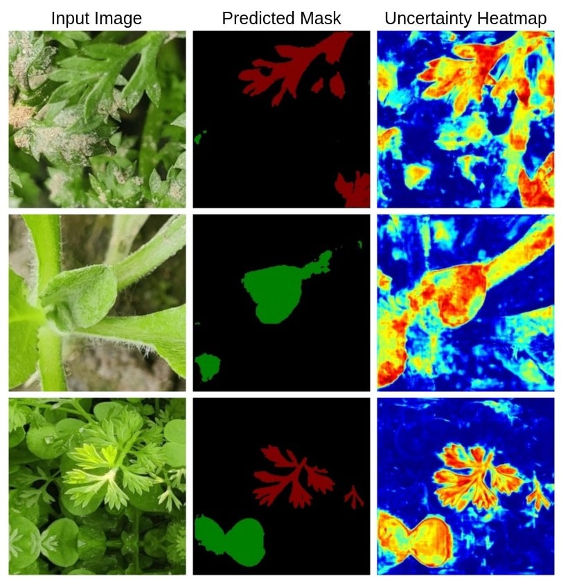
Before diving into the visual comparison, let’s quickly decode what the colors in the heatmaps represent:
- Blue: Low uncertainty — the model is confident in its prediction.
- Yellow: Moderate uncertainty — the model is unsure and the prediction may need review.
- Red: High uncertainty — the model is highly unsure, often indicating noise, ambiguity, or out-of-distribution patterns.
These heatmaps are generated using Monte Carlo Dropout, where each pixel’s color is based on the standard deviation across multiple stochastic predictions.
Side-by-Side Heatmap Comparison
In the figure below, each row represents a test image. The columns show:
- Input Image
- Uncertainty Heatmap (Approach 1: Inject Dropout)
- Uncertainty Heatmap (Approach 2: Train with Dropout)
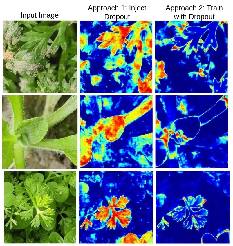
Key Observations:
- Approach 1 (Middle Column) shows more widespread uncertainty, including noisy areas in the background. Since dropout is added post-training, the model isn’t trained to handle it, leading to more diffuse uncertainty.
- Approach 2 (Right Column) produces sharper and more structured heatmaps. The model, having seen dropout during training, learns to be confident in clear areas and only uncertain at complex or ambiguous boundaries.
This visual difference highlights why training with dropout can lead to more calibrated and localized uncertainty estimates.
Conclusion: Trustworthy AI Begins with Knowing What You Don’t Know
As deep learning systems grow in complexity and responsibility, knowing what your model predicts is no longer enough — you must know how sure it is. With Monte Carlo Dropout, we can bring this capability to segmentation models like UNet with minimal architectural changes.
Both approaches explored in this tutorial offer practical ways to incorporate uncertainty estimation into your workflows:
- Approach 1 (Inject Dropout): Fast, flexible, works with pre-trained models.
- Approach 2 (Train with Dropout): More stable and precise uncertainty, especially near object boundaries.
With Uncertainty Estimation, you’re not just building accurate models — you’re building reliable and explainable ones.
FAQs & Common Pitfalls
Q1: Why is the uncertainty map noisy in Approach 1?
Because the model wasn’t trained with dropout, it hasn’t learned to be robust to random neuron deactivation. That’s why Approach 2 usually results in cleaner heatmaps.
Q2: How many stochastic passes (T) should I use?
Generally, 20–50 passes provide a good trade-off between quality and speed. More passes give smoother uncertainty, but take longer to compute.
Q3: Can this be applied to architectures other than UNet?
Absolutely! You can apply the same principles to DeepLabV3+, FPN, or even transformers like SegFormer — just identify where to add or activate dropout layers in the decoder.
Q4: Do I need to modify the loss function?
No. The loss function (e.g., CrossEntropyLoss) remains the same. Uncertainty is derived from model predictions, not loss modifications.
Resources and Next Steps
Ready to explore further? Here’s where to go next:
Watch the Full YouTube Tutorial: Uncertainty Estimation in Image Segmentation using Monte Carlo Dropout – PyTorch Tutorial
Access the Codebase on GitHub: Multiclass Segmentation in PyTorch
Suggested Reading:
- Yarin Gal & Zoubin Ghahramani (2016). Dropout as a Bayesian Approximation: Representing Model Uncertainty in Deep Learning.
- Kendall & Gal (2017). What Uncertainties Do We Need in Bayesian Deep Learning for Computer Vision?
Try Next:
- Aleatoric vs Epistemic Uncertainty
- Combining MC Dropout with Grad-CAM for explainability
- Using uncertainty maps for active dataset selection