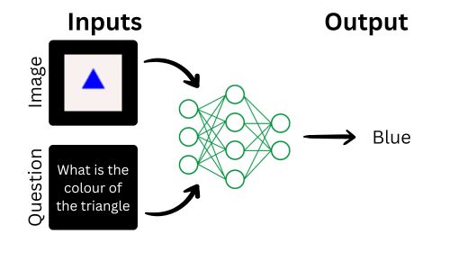
Visual Question Answering from Scratch using TensorFlow

Visual Question Answering (VQA) is a fascinating field in artificial intelligence where a system answers questions about an image. This combines natural language processing (NLP) to understand the question and computer vision to analyze the image. For example, given an image of a red apple and the question “What color is the fruit?”, the model would answer “Red.”

Project Overview

In this project, we’ll build a simple Visual Question Answering model using the Easy VQA dataset. Easy VQA is designed to help beginners get started with VQA by offering a small, manageable dataset. Our implementation will involve:

Understanding the dataset: Exploring its structure and contents.
Preprocessing the data: Preparing the dataset for training.
Building a model in TensorFlow: Creating a model that integrates visual and textual inputs.
Training and evaluating the model: Using Easy VQA’s training and testing sets.
Visualizing results: Showcasing how the model predicts answers for test images and questions.

READ MORE:

Dataset: Easy VQA

Easy VQA is a beginner-friendly dataset for Visual Question Answering. It includes:

4,000 training images and 38,575 training questions.
1,000 test images and 9,673 test questions.
A total of 13 possible answers.
Many questions are binary yes/no types:
- 28,407 yes/no questions in the training set.
- 7,136 yes/no questions in the testing set.

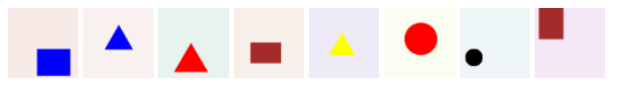
All images are 64×64 color images, making them lightweight and easy to work with.

For more: Easy VQA

The dataset is small enough to be trained on a regular computer with a modest GPU, making it perfect for beginners and small-scale experimentation.

Code: https://github.com/nikhilroxtomar/Visual-Question-Answer

Dataset Preprocessing

Here, we’ll load the dataset, split it into training and validation sets, and process the images and questions.

Loading Dataset

We define functions to load the questions, answers, and image paths.

import os
import numpy as np
import cv2
from glob import glob
import json
from sklearn.model_selection import train_test_split

First of all, let us import all the libraries and functions that will be required.

def get_data(dataset_path, train=True):
    # Determine if we are processing training or testing data
    data_type = "train" if train else "test"

    # Load questions and answers from the JSON file
    with open(os.path.join(dataset_path, data_type, "questions.json"), "r") as file:
        data = json.load(file)

    questions, answers, image_paths = [], [], []
    # Parse the questions, answers, and corresponding image paths
    for q, a, p in data:
        questions.append(q)
        answers.append(a)
        image_paths.append(os.path.join(dataset_path, data_type, "images", f"{p}.png"))

    return questions, answers, image_paths

The function reads a JSON file containing questions, answers, and image names. It returns three lists:

questions: A list of textual questions.
answers: The corresponding answers.
image_paths: Full paths to the associated images.

Getting Unique Answer Labels

We load the unique set of 13 possible answers:

def get_answers_labels(dataset_path):
    with open(os.path.join(dataset_path, "answers.txt"), "r") as file:
        data = file.read().strip().split("\n")
        return data

This function reads a file answers.txt, which lists all possible answers (like “yes”, “no”, “red”, etc.). It splits the file into a list of answers

Splitting Data into Train, Validation, and Test Sets

def main():
    dataset_path = "data"
    
    # Load training and testing data
    trainQ, trainA, trainI = get_data(dataset_path, train=True)
    testQ, testA, testI = get_data(dataset_path, train=False)
    unique_answers = get_answers_labels(dataset_path)

    # Split the training data into training and validation sets
    trainQ, valQ, trainA, valA, trainI, valI = train_test_split(
        trainQ, trainA, trainI, test_size=0.2, random_state=42
    )

    # Print statistics
    print(f"Train -> Questions: {len(trainQ)} - Answers: {len(trainA)} - Images: {len(trainI)}")
    print(f"Valid -> Questions: {len(valQ)} - Answers: {len(valA)} - Images: {len(valI)}")
    print(f"Test -> Questions: {len(testQ)} - Answers: {len(testA)} - Images: {len(testI)}")

In the main function, we execute all the functions present in the data processing part.

Load Training and Testing Data

Training data: Loaded using get_data(dataset_path, train=True).
Testing data: Loaded using get_data(dataset_path, train=False).

Split Training Data into Training and Validation

train_test_split divides the training dataset into:
- Training set (80%): Used for model learning.
- Validation set (20%): Used to check how well the model generalizes during training.

Print Statistics

Helps verify the size of each dataset (train, validation, and test).

Output Example

Train -> Questions: 30860 - Answers: 30860 - Images: 30860
Valid -> Questions: 7715 - Answers: 7715 - Images: 7715
Test -> Questions: 9673 - Answers: 9673 - Images: 9673

Model Implementation

The model can be divided into three key components:

Vision Part (CNN): Processes the image input to extract features.
NLP Part (MLP): Processes the question input to extract features.
Merge and Output Part: Combines the features from the vision and NLP parts and generates the final answer.

Import the TensorFlow Framework

from tensorflow.keras import layers as L
from tensorflow.keras import Model

Vision Part (CNN)

This sub-network processes the image input (image_shape=(64, 64, 3)) using a Convolutional Neural Network (CNN).

# Vision Part: Image Processing
image_input = L.Input(image_shape)

# Convolutional layers with max pooling and ReLU activation
x1 = L.Conv2D(8, 3, padding='same')(image_input)
x1 = L.MaxPooling2D()(x1)
x1 = L.Activation("relu")(x1)

x1 = L.Conv2D(16, 3, padding='same')(x1)
x1 = L.MaxPooling2D()(x1)
x1 = L.Activation("relu")(x1)

# Flatten the feature map and apply a Dense layer
x1 = L.Flatten()(x1)
x1 = L.Dense(32, activation='tanh')(x1)

Conv2D Layers: Extract spatial features from the image.
MaxPooling2D: Down-samples the feature maps to reduce dimensions and capture important features.
Flatten: Converts the 2D feature maps into a 1D vector for the fully connected layers.
Dense Layer: Reduces the feature representation to a size of 32 and uses an tanh activation for non-linearity.

NLP Part (MLP)

This sub-network processes the question input (vocab_size=27) using a Multi-Layer Perceptron (MLP).

# NLP Part: Question Processing
question_input = L.Input(shape=(vocab_size,))

# Dense layers with tanh activation
x2 = L.Dense(32, activation='tanh')(question_input)
x2 = L.Dense(32, activation='tanh')(x2)

Input Layer: The question input is represented as a one-hot encoded vector with a size equal to the vocabulary size (vocab_size=27).
Dense Layers: Two fully connected layers with tanh activation extract meaningful features from the question input.

Merge and Output Part

This sub-network combines the features from the vision and NLP parts and generates the final prediction.

# Merge Vision and NLP Parts
out = L.Multiply()([x1, x2])  # Element-wise multiplication of features

# Dense layers to combine features and generate predictions
out = L.Dense(32, activation='tanh')(out)
out = L.Dense(num_answers, activation='softmax')(out)

Multiply Layer: Combines the image and question features using element-wise multiplication. This operation models the interaction between visual and textual features.
Dense Layers: Further process the combined features.
- The first Dense layer with tanh activation refines the combined representation.
- The second Dense layer with softmax activation outputs probabilities for each of the possible answers (num_answers=13).

Final Model Assembly

The complete model integrates the three components:

model = Model(inputs=[image_input, question_input], outputs=out)

Inputs: The model takes two inputs:
- image_input (image features).
- question_input (question features).

Output: The model predicts the answer as a probability distribution over 13 possible answers.

Training the VQA Model

We first begin by importing all the required libraries and functions.

import os
import numpy as np
import cv2
import tensorflow as tf
from tensorflow.keras.preprocessing.text import Tokenizer
from tensorflow.keras.optimizers import Adam
from tensorflow.keras.callbacks import ModelCheckpoint, ReduceLROnPlateau, EarlyStopping, CSVLogger
from sklearn.model_selection import train_test_split
from data import get_data, get_answers_labels
from model import build_model

The create_dir function is used to create a directory which is used to save the files.

def create_dir(path):
    if not os.path.exists(path):
        os.makedirs(path)

Dataset Preparation

The TFDataset class is responsible for parsing the raw data into a format suitable for TensorFlow training.

class TFDAtaset:
    def __init__(self, tokenizer, labels, image_h, image_w):
        self.tokenizer = tokenizer
        self.labels = labels
        self.image_h = image_h
        self.image_w = image_w

    def parse(self, question, answer, image_path):
        question = question.decode()
        answer = answer.decode()
        image_path = image_path.decode()

        """ Question """
        question = self.tokenizer.texts_to_matrix([question])
        question = np.array(question[0], dtype=np.float32)

        """ Answer """
        index = self.labels.index(answer)
        answer = [0] * len(self.labels)
        answer[index] = 1
        answer = np.array(answer, dtype=np.float32)

        """ Image """
        image = cv2.imread(image_path, cv2.IMREAD_COLOR)
        image = cv2.resize(image, (self.image_w, self.image_h))
        image = image/255.0
        image = image.astype(np.float32)

        return question, answer, image


    def tf_parse(self, question, answer, image_path):
        q, a, i = tf.numpy_function(
            self.parse,
            [question, answer, image_path],
            [tf.float32, tf.float32, tf.float32]
        )
        q.set_shape([len(self.tokenizer.word_index) + 1,])
        a.set_shape([len(self.labels),])
        i.set_shape([self.image_h, self.image_w, 3])

        return (i, q), a

    def tf_dataset(self, questions, answers, image_paths, batch_size=16):
        ds = tf.data.Dataset.from_tensor_slices((questions, answers, image_paths))
        ds = ds.map(self.tf_parse).batch(batch_size).prefetch(10)
        return ds

parse(): Converts the question, answer, and image path into numerical representations.

Question: Tokenized into a bag-of-words representation.
Answer: One-hot encoded based on the label index.
Image: Loaded, resized, and normalized to pixel values in the range [0, 1].

tf_parse(): Wraps parse() for compatibility with TensorFlow datasets using tf.numpy_function.

tf_dataset(): Creates a batched and pre-fetched TensorFlow dataset.

Seeding and parameters

""" Seeding """
tf.random.set_seed(42)

""" Directory for storing files """
create_dir("files")

""" Hyperparameters """
image_shape = (64, 64, 3)
batch_size = 32
num_epochs = 20

model_path = os.path.join("files", "model.h5")
csv_path = os.path.join("files", "data.csv")

Training Pipeline

Fetch the dataset and split it into training and validation set.
Tokenizer: Converts text questions into numerical formats.
Dataset Pipeline: TFDataset prepares training and validation datasets.

dataset_path = "data"
trainQ, trainA, trainI = get_data(dataset_path, train=True)
testQ, testA, testI = get_data(dataset_path, train=False)
unique_answers = get_answers_labels(dataset_path)
num_answers = len(unique_answers)

""" Split the data into training and validation """
trainQ, valQ, trainA, valA, trainI, valI = train_test_split(
    trainQ, trainA, trainI, test_size=0.2, random_state=42
)

tokenizer = Tokenizer()
tokenizer.fit_on_texts(trainQ + valQ)
vocab_size = len(tokenizer.word_index) + 1

ds = TFDAtaset(tokenizer, unique_answers, image_h=image_shape[0], image_w=image_shape[1])
train_ds = ds.tf_dataset(trainQ, trainA, trainI, batch_size=batch_size)
valid_ds = ds.tf_dataset(valQ, valA, valI, batch_size=batch_size)

Model Building

model = build_model(image_shape=image_shape, vocab_size=vocab_size, num_answers=num_answers)
model.compile(
    optimizer=Adam(learning_rate=5e-4),
    loss='categorical_crossentropy',
    metrics=['accuracy']
)

Callbacks for Training

The following callbacks are defined:

ModelCheckpoint: Saves the best model based on validation loss.
ReduceLROnPlateau: Reduces the learning rate if validation loss plateaus.
CSVLogger: Logs training metrics to a CSV file.
EarlyStopping: Stops training if no improvement in validation loss.

callbacks = [
    ModelCheckpoint(model_path, monitor='val_loss', verbose=1, save_best_only=True),
    ReduceLROnPlateau(monitor='val_loss', factor=0.1, patience=5, min_lr=1e-7, verbose=1),
    CSVLogger(csv_path, append=True),
    EarlyStopping(monitor='val_loss', patience=20, restore_best_weights=False)
]

Training the Model

The model is trained using the prepared datasets and callbacks.

model.fit(
    train_ds,
    validation_data=valid_ds,
    epochs=num_epochs,
    callbacks=callbacks
)

Evaluating and Visualizing Test Results

Finally, we evaluate the trained model’s performance on a test dataset and produce a classification report and a confusion matrix visualization.

Imports

import os
import matplotlib.pyplot as plt
import seaborn as sns
import numpy as np
import cv2
from tqdm import tqdm
import tensorflow as tf
from tensorflow.keras.preprocessing.text import Tokenizer
from sklearn.model_selection import train_test_split
from sklearn.metrics import classification_report, confusion_matrix, ConfusionMatrixDisplay
from data import get_data, get_answers_labels

Seeding and Parameters

""" Seeding """
tf.random.set_seed(42)

""" Parameters """
image_shape = (64, 64)
model_path = os.path.join("files", "model.h5")

Dataset Loading and Processing

""" Split the data into training and validation """
trainQ, valQ, trainA, valA, trainI, valI = train_test_split(
    trainQ, trainA, trainI, test_size=0.2, random_state=42
)

print(f"Train -> Questions: {len(trainQ)} - Answers: {len(trainA)} - Images: {len(trainI)}")
print(f"Valid -> Questions: {len(valQ)} - Answers: {len(valA)} - Images: {len(valI)}")
print(f"Test -> Questions: {len(testQ)} - Answers: {len(testA)} - Images: {len(testI)}")

""" Tokenizer: BOW """
tokenizer = Tokenizer()
tokenizer.fit_on_texts(trainQ + valQ)
vocab_size = len(tokenizer.word_index) + 1

testQ = tokenizer.texts_to_matrix(testQ)

Loading Model

model = tf.keras.models.load_model("files/model.h5")

Evaluation Loop

Iterates over the test dataset to make predictions and collect true and predicted values.

true_values, pred_values = [], []
for question, answer, image_path in tqdm(zip(testQ, testA, testI), total=len(testQ)):
    """ Question """
    question = np.expand_dims(question, axis=0)

    """ Answer """
    answer = unique_answers.index(answer)
    true_values.append(answer)

    """ Image """
    image = cv2.imread(image_path, cv2.IMREAD_COLOR)
    image = cv2.resize(image, image_shape)
    image = image/255.0
    image = image.astype(np.float32)
    image = np.expand_dims(image, axis=0)

    """ Prediction """
    pred = model.predict([image, question], verbose=0)[0]
    pred = np.argmax(pred, axis=-1)
    pred_values.append(pred)

Evaluation and Visualization

""" Classification Report """
report = classification_report(true_values, pred_values, target_names=unique_answers)
print(report)

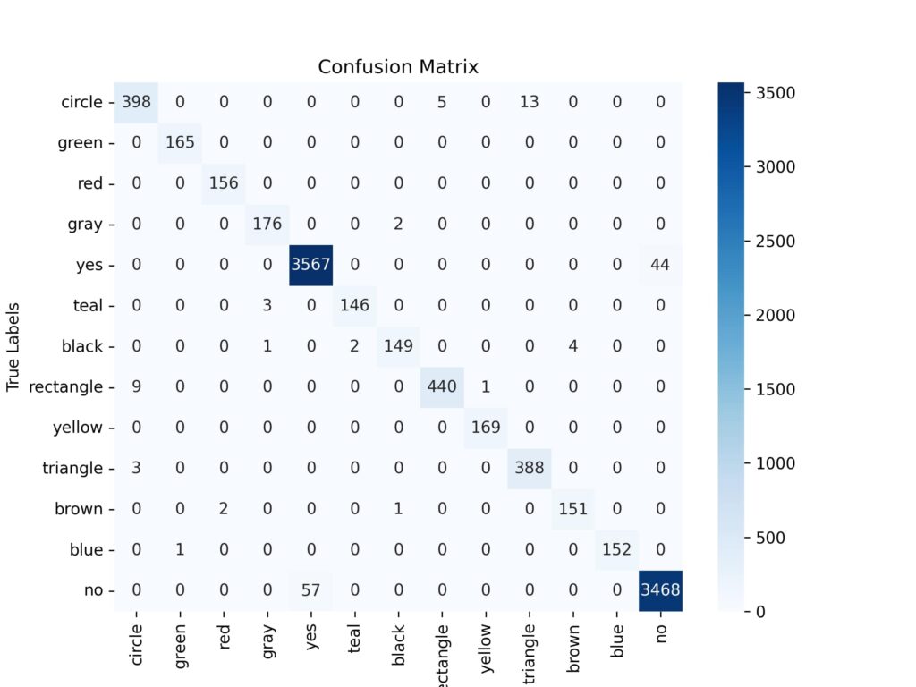
""" Confusion Matrix """
 cm = confusion_matrix(true_values, pred_values)

plt.figure(figsize=(8, 6))
sns.heatmap(cm, annot=True, fmt='d', cmap='Blues', xticklabels=unique_answers, yticklabels=unique_answers)
plt.title('Confusion Matrix')
plt.xlabel('Predicted Labels')
plt.ylabel('True Labels')

plt.savefig('files/confusion_matrix_heatmap.png', dpi=300)
plt.close()

Output:

Generates a detailed classification report, including precision, recall, F1-score, and support for each class.

              precision    recall  f1-score   support

      circle       0.97      0.96      0.96       416
       green       0.99      1.00      1.00       165
         red       0.99      1.00      0.99       156
        gray       0.98      0.99      0.98       178
         yes       0.98      0.99      0.99      3611
        teal       0.99      0.98      0.98       149
       black       0.98      0.96      0.97       156
   rectangle       0.99      0.98      0.98       450
      yellow       0.99      1.00      1.00       169
    triangle       0.97      0.99      0.98       391
       brown       0.97      0.98      0.98       154
        blue       1.00      0.99      1.00       153
          no       0.99      0.98      0.99      3525

    accuracy                           0.98      9673
   macro avg       0.98      0.98      0.98      9673
weighted avg       0.98      0.98      0.98      9673

Confusion Matrix: It shows the relationship between true and predicted labels using a confusion matrix and shows it in the form of heatmap using seaborn.

The confusion matrix shows the performance of the classes on the Easy VQA (Visual Question Answer) test set

Conclusion

In this tutorial, we walked through a complete pipeline for evaluating a trained multi-modal model using a test dataset comprising questions, answers, and images. Starting with data preprocessing, including tokenizing questions and resizing images, we then loaded the pre-trained model to generate predictions. Using true and predicted labels, we calculated key performance metrics, including a classification report and a confusion matrix, which were visualized for better understanding.

Idiot Developer