Deep learning models, especially convolutional neural networks (CNNs), often function as black boxes, making it difficult to interpret their decision-making processes. Gradient-weighted Class Activation Mapping (GradCAM) is a powerful technique used to visualize and understand these models by highlighting the regions of an image that contribute most to a prediction.

This article provides a step-by-step guide to implementing GradCAM in PyTorch using MobileNetV2, enabling better model interpretability.

What is GradCAM?

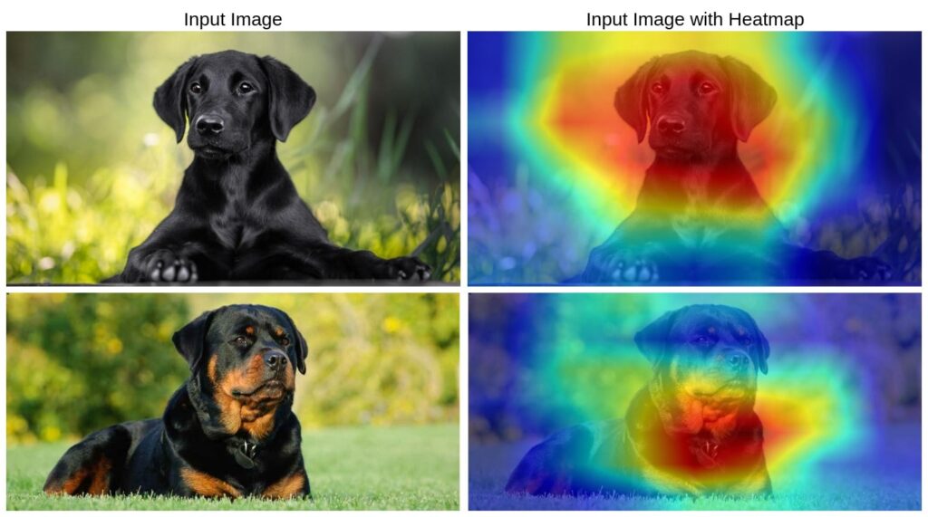
Gradient-weighted Class Activation Mapping (GradCAM) is used to interpret and visualize deep learning models, especially convolutional neural networks (CNNs). It highlights the regions of an input image most important for a model’s prediction. This is done by computing the gradients of the target class score concerning the final convolutional layer of the model. The resulting heatmap provides insight into why the model made a specific prediction.

Read More

• GradCAM with TensorFlow: Interpreting Neural Networks with Class Activation Maps

Core Idea and Architecture

GradCAM works by leveraging the gradients of a target class flowing into the final convolutional layer of a CNN. The core steps involved in GradCAM are:

1. Forward Pass: The input image is passed through the network to obtain predictions.
2. Backward Pass: The gradients of the target class concerning the feature maps of the final convolutional layer are computed.
3. Weight Calculation: The gradients are globally pooled to obtain a set of weights.
4. Heatmap Generation: The weighted sum of the feature maps is computed, followed by applying a ReLU function to discard negative values.
5. Overlaying Heatmap: The heatmap is superimposed onto the original image for visualization.

By using this method, GradCAM helps us understand which regions contribute the most to a model’s decision.

Advantages

• Model Interpretability: Helps in visualizing which parts of an image influence the model’s prediction.
• Debugging: Useful for identifying incorrect predictions and potential biases in the model.
• Generalization: Can be applied to various CNN architectures like MobileNet, ResNet, and VGG.
• No Model Modification: Does not require changes to the original model structure.

Implementation

Below is a step-by-step implementation of GradCAM in PyTorch using MobileNetV2.

Import Required Libraries

import os
import numpy as np
import cv2
import torch
import torchvision.transforms as transforms
from torchvision import models

Preprocessing the Image

def preprocess_image(img_path):
    img = cv2.imread(img_path, cv2.IMREAD_COLOR)
    img = cv2.resize(img, (224, 224))  # Resize for MobileNetV2
    img = transforms.ToTensor()(img)
    img = transforms.Normalize(mean=[0.485, 0.456, 0.406], std=[0.229, 0.224, 0.225])(img)
    img = img.unsqueeze(0)  # Add batch dimension
    return img

This function reads and preprocesses an image by resizing it to 224×224, normalizing it, and adding a batch dimension.

Getting the Class Label

def get_class_label(preds):
    _, class_index = torch.max(preds, 1)
    return class_index.item()

This function extracts the class index with the highest probability from model predictions.

Extracting the Convolutional Layer

def get_conv_layer(model, conv_layer_name):
    for name, layer in model.named_modules():
        if name == conv_layer_name:
            return layer
    raise ValueError(f"Layer '{conv_layer_name}' not found in the model.")

This function retrieves a specified convolutional layer from the model.

Computing Grad-CAM Heatmap

def compute_gradcam(model, img_tensor, class_index, conv_layer_name="features.18"):
    conv_layer = get_conv_layer(model, conv_layer_name)

    # Forward hook to store activations
    activations = None
    def forward_hook(module, input, output):
        nonlocal activations
        activations = output

    hook = conv_layer.register_forward_hook(forward_hook)

    # Compute gradients
    img_tensor.requires_grad_(True)
    preds = model(img_tensor)
    loss = preds[:, class_index]
    model.zero_grad()
    loss.backward()

    # Get gradients
    grads = img_tensor.grad.cpu().numpy()
    pooled_grads = np.mean(grads, axis=(0, 2, 3))

    # Remove the hook
    hook.remove()

    activations = activations.detach().cpu().numpy()[0]
    for i in range(pooled_grads.shape[0]):
        activations[i, ...] *= pooled_grads[i]

    heatmap = np.mean(activations, axis=0)
    heatmap = np.maximum(heatmap, 0)
    heatmap /= np.max(heatmap)

    return heatmap

In this step, we generate the heatmap that highlights the important regions in the image for the model’s prediction. The function compute_gradcam follows these steps:

1. Retrieve the convolutional layer: We extract the last convolutional layer from MobileNetV2 (typically features.18) since GradCAM relies on convolutional feature maps.
2. Register a forward hook: This hook captures the activations (feature maps) of the last convolutional layer when the image is passed through the model.
3. Compute gradients:
   • The input image is set to require gradients.
   • We perform a forward pass through the model to get predictions.
   • The loss is computed based on the class index corresponding to the highest prediction score.
   • A backward pass is performed to compute gradients concerning the feature maps.
4. Compute importance weights: The gradients are averaged across spatial dimensions (height and width), resulting in a weight for each feature map.
5. Generate the heatmap:
   • The feature maps are multiplied by their respective weights.
   • The sum of weighted feature maps is taken.
   • ReLU activation is applied to remove negative values.
   • The heatmap is normalized between 0 and 1.

This heatmap highlights the most influential parts of the image for the model’s prediction.

Overlaying Heatmap on Image

def overlay_heatmap(img_path, heatmap, alpha=0.4):
    img = cv2.imread(img_path, cv2.IMREAD_COLOR)
    heatmap = cv2.resize(heatmap, (img.shape[1], img.shape[0]))
    heatmap = np.uint8(255 * heatmap)
    heatmap = cv2.applyColorMap(heatmap, cv2.COLORMAP_JET)

    superimposed_img = cv2.addWeighted(img, alpha, heatmap, 1 - alpha, 0)
    return superimposed_img

Once we generate the heatmap, we overlay it onto the original image to create a visually interpretable output. The function overlay_heatmap performs the following steps:

1. Resize the heatmap: The GradCAM heatmap is resized to match the dimensions of the input image.
2. Convert heatmap to color: The values in the heatmap (ranging from 0 to 1) are mapped to a COLORMAP_JET, where high values appear in red and low values in blue.
3. Blend heatmap with the original image:
   • The color heatmap is superimposed on the input image.
   • A blending factor (alpha) controls the transparency of the heatmap.
   • The resulting visualization shows which regions influenced the model’s decision the most.

Running the Implementation

if __name__ == "__main__":
    # Load a pretrained model (MobileNetV2)
    model = models.mobilenet_v2(pretrained=True)
    model.eval()

    # Example Usage
    img_path = "images/dog-2.jpg"  # Replace with your image path
    img_tensor = preprocess_image(img_path)

    # Get model predictions
    with torch.no_grad():
        preds = model(img_tensor)
    class_index = get_class_label(preds)

    print(f"Predicted Class Index: {class_index}")

    # Compute Grad-CAM heatmap
    heatmap = compute_gradcam(model, img_tensor, class_index)

    # Overlay heatmap on the original image
    output_img = overlay_heatmap(img_path, heatmap)

    # Save the heatmap
    cv2.imwrite("heatmap/2.jpg", output_img)

This section ties everything together and executes the full GradCAM process:

1. Load the Pretrained Model: MobileNetV2 is loaded with pretrained weights, and the model is set to evaluation mode.
2. Preprocess the Input Image:
   • The input image is read and resized.
   • It is converted to a tensor and normalized to match the expected format for MobileNetV2.
3. Perform Model Inference:
   • The preprocessed image is passed through the model.
   • The class with the highest probability is selected.
4. Compute GradCAM Heatmap: The computed heatmap highlights the regions most relevant to the selected class.
5. Overlay the Heatmap: The heatmap is blended with the original image for visualization.
6. Save the Output: The final image with the overlay is saved as an output file.

Conclusion

GradCAM is a powerful interpretability technique for deep learning models, particularly CNNs. It allows us to visualize which regions in an image influence a model’s decision, making AI models more transparent. By implementing GradCAM in PyTorch with MobileNetV2, we can analyze model predictions effectively.

Read More

• Implementing Grad-CAM in PyTorch
• Grad-CAM: Visualize class activation maps with Keras, TensorFlow, and Deep Learning