GradCAM Heatmaps for Segmentation with UNet in PyTorch

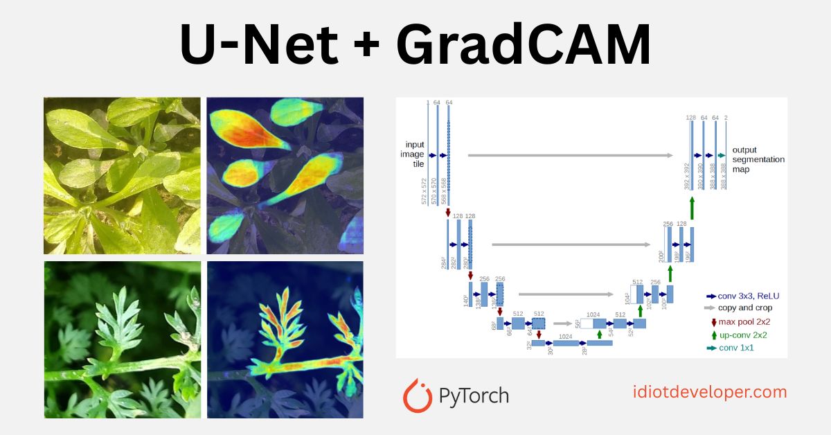
In semantic segmentation, understanding how a deep learning model arrives at its decisions is crucial—especially in fields like medical imaging, agriculture, and autonomous systems. While U-Net and other architectures can deliver high accuracy, they often act as black boxes. In this blog post, we go beyond prediction accuracy. We’ll visualize where the model focuses for each class prediction using GradCAM (Gradient-weighted Class Activation Mapping). This will help you:

• Diagnose model behavior
• Understand failure cases
• Communicate your results visually

We’ll build on a U-Net trained for multiclass segmentation in PyTorch and use GradCAM to generate per-class heatmaps overlaid on the original image.

What is Multiclass Segmentation?

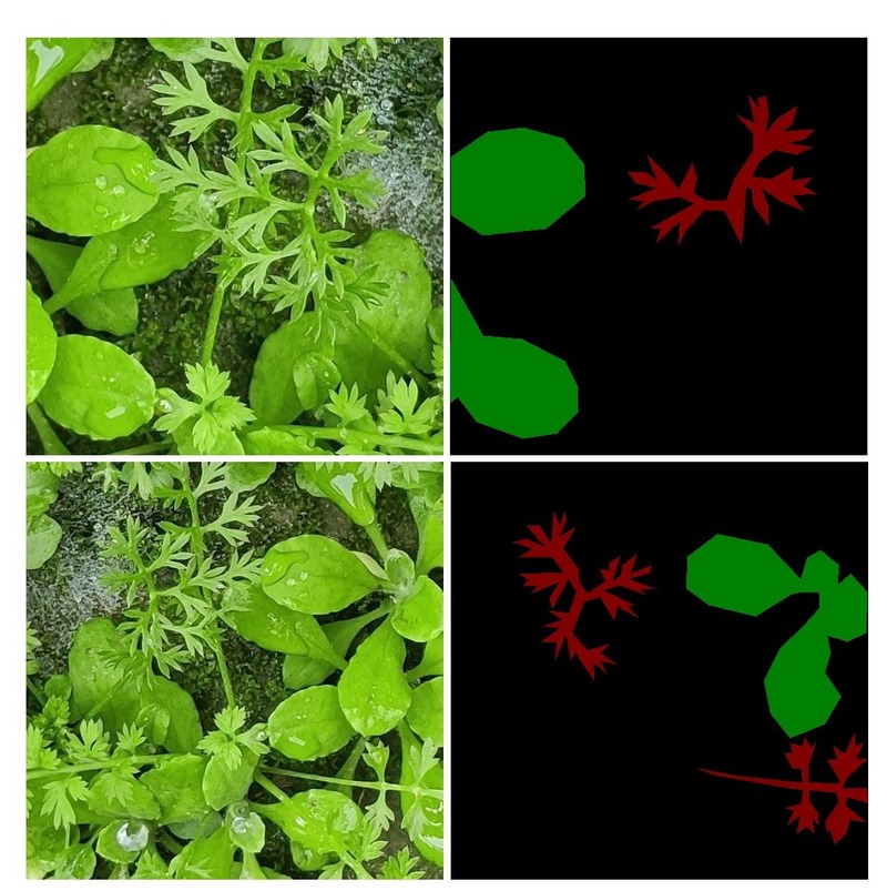
Multiclass segmentation is a computer vision task where every pixel in an image is classified into one of several categories. Unlike binary segmentation (foreground vs background), multiclass segmentation predicts one of n classes for each pixel.

For instance, in a weed detection task, we may want to segment:

• Background
• Weed Type 1
• Weed Type 2

Each of these is a mutually exclusive class, and the model must assign a pixel to only one of them.

What is GradCAM?

GradCAM (Gradient-weighted Class Activation Mapping) is a technique to generate visual explanations for deep learning models, especially CNNs.

It works by:

1. Computing gradients of a target output (e.g., class score) with respect to feature maps of a convolutional layer.
2. Weighing those feature maps based on the gradients.
3. Creating a coarse heatmap indicating the “important” regions in the input image.

In segmentation, we apply GradCAM per class, enabling us to see where the model “looks” when predicting a particular class.

Implementation

Let’s walk through how to add GradCAM-based heatmap visualizations to your multiclass segmentation model.

Imports and Setup

First, we import all the required libraries.

import os
import time
import numpy as np
import cv2
from tqdm import tqdm
import torch
import torch.nn.functional as F

from model import build_unet
from utils import create_dir, seeding
from train import load_data

Fetching the Convolutional Layer

def get_conv_layer(model, conv_layer_name):
    for name, layer in model.named_modules():
        if name == conv_layer_name:
            return layer
    raise ValueError(f"Layer '{conv_layer_name}' not found in the model.")

This helper function finds the target convolutional layer (by name) from your U-Net model, which we’ll use to compute GradCAM.

Arguments:

• model: The PyTorch model (U-Net in this case).
• conv_layer_name: String name of the layer (e.g., “d4.conv.conv.5”).

How it works:

It loops through all named submodules in the model and returns the one that matches conv_layer_name. If not found, it raises an error.

Computing GradCAM for Segmentation

def compute_segmentation_gradcam(model, image_tensor, target_class, conv_layer_name=None):
    ## Finds the layer
    conv_layer = get_conv_layer(model, conv_layer_name)
    activations = []
    gradients = []

    ## Define hooks
    def forward_hook(module, input, output):
        activations.append(output)

    def backward_hook(module, grad_in, grad_out):
        gradients.append(grad_out[0])

    ## Forward hook saves output feature maps of the chosen layer.
 ## Backward hook captures the gradients of the layer’s output during backpropagation.

    forward_handle = conv_layer.register_forward_hook(forward_hook)
    backward_handle = conv_layer.register_backward_hook(backward_hook)

    ## Make prediction and get class-specific score
    output = model(image_tensor)
    probs = torch.softmax(output, dim=1)
    target = probs[0, target_class, :, :].mean()

    ## Backpropagate to compute gradients
    model.zero_grad()
    target.backward()

    grads_val = gradients[0].detach()[0]
    acts_val = activations[0].detach()[0]

    ## Compute channel-wise weights and generate Grad-CAM
    weights = grads_val.mean(dim=(1, 2))
    gradcam = torch.zeros(acts_val.shape[1:], dtype=torch.float32).to(image_tensor.device)
    for i, w in enumerate(weights):
        gradcam += w * acts_val[i]

    ## Generate Grad-CAM map
    gradcam = F.relu(gradcam)
    gradcam = gradcam - gradcam.min()
    gradcam = gradcam / (gradcam.max() + 1e-8)
    gradcam = gradcam.cpu().numpy()

    ## Clean up: remove hooks
    forward_handle.remove()
    backward_handle.remove()
    return gradcam

The above function generates the GradCAM heatmap for a specific class in a multiclass segmentation task.

Arguments:

• model: Your trained U-Net model.
• image_tensor: Input image tensor of shape [1, C, H, W].
• target_class: Class index for which to compute the GradCAM.
• conv_layer_name: The name of the intermediate convolutional layer to visualize.

How it works:

1. Retrieve the layer: Calls get_conv_layer() to fetch the convolutional layer.
2. Register Hooks: 
   • forward_hook stores the activations.
   • backward_hook stores the gradients with respect to the output of the chosen conv layer.
3. Forward Pass: Runs the model to get the softmax probabilities. Selects the average of the output for the target_class.
4. Backward Pass: Backpropagates from the selected class probability to compute gradients.
5. Generate GradCAM:
   • Averages gradients across spatial dimensions to get weights.
   • Performs a weighted sum of activations to produce a raw heatmap.
   • Applies ReLU, normalizes the heatmap to [0, 1].
6. Cleanup: Removes the forward and backward hooks to avoid memory leaks.

Output: Returns a 2D NumPy array representing the heatmap.

Overlaying the Heatmap

def overlay_heatmap_on_image(image_np, heatmap, alpha=0.4):
    heatmap = cv2.resize(heatmap, (image_np.shape[1], image_np.shape[0]))
    heatmap = np.uint8(255 * heatmap)
    heatmap = cv2.applyColorMap(heatmap, cv2.COLORMAP_JET)
    superimposed_img = cv2.addWeighted(image_np, alpha, heatmap, 1 - alpha, 0)
    return superimposed_img

The function blends the GradCAM heatmap with the original image to visually highlight regions of focus.

Arguments:

• image_np: The original image as a NumPy array (HWC format).
• heatmap: The GradCAM heatmap array (2D, normalized).
• alpha: Blending ratio between the image and the heatmap.

How it works:

1. Resizes the heatmap to match the image size.
2. Converts the heatmap to a colored image using OpenCV’s COLORMAP_JET.
3. Overlays it on top of the original image using cv2.addWeighted.

Output: A NumPy array of the heatmap-superimposed image.

Applying GradCAM to the Dataset

def apply_gradcam(model, save_path, test_x, test_y, size, colormap, layer=None):
    for i, (x_path, y_path) in tqdm(enumerate(zip(test_x, test_y)), total=len(test_x)):
        name = os.path.basename(x_path).split(".")[0]

        image = cv2.imread(x_path, cv2.IMREAD_COLOR)
        image = cv2.resize(image, size)
        save_img = image.copy()

        input_image = np.transpose(image, (2, 0, 1)) / 255.0
        input_image = np.expand_dims(input_image, axis=0).astype(np.float32)
        input_tensor = torch.from_numpy(input_image).to(device)

        mask = cv2.imread(y_path, cv2.IMREAD_COLOR)
        mask = cv2.resize(mask, size)

        for class_idx in range(len(colormap)):
            gradcam = compute_segmentation_gradcam(model, input_tensor, class_idx, conv_layer_name=layer)
            cam_img = overlay_heatmap_on_image(save_img.copy(), gradcam)

            class_rgb = np.array(colormap[class_idx], dtype=np.uint8)
            binary_mask = cv2.inRange(mask, class_rgb, class_rgb)
            binary_mask = cv2.cvtColor(binary_mask, cv2.COLOR_GRAY2BGR)

            line = np.ones((size[1], 10, 3), dtype=np.uint8) * 255
            combined_img = np.concatenate([save_img, line, cam_img, line, binary_mask], axis=1)

            cam_dir = f"{save_path}/gradcam/{class_idx}"
            os.makedirs(cam_dir, exist_ok=True)
            cv2.imwrite(f"{cam_dir}/{name}.jpg", combined_img)

The function applies GradCAM to a batch of test images and saves the visual results.

Arguments:

• model: Trained U-Net model.
• save_path: Directory to save output visualizations.
• test_x: List of test image file paths.
• test_y: List of corresponding mask file paths.
• size: Tuple (width, height) to resize input.
• colormap: List of RGB values for each class.
• layer: The name of the convolutional layer for GradCAM.

How it works:

1. Iterates over test images.
2. Loads and preprocesses each image and its mask.
3. For each class:

• Computes GradCAM heatmap.
• Overlay it on the input image.
• Extracts the binary ground-truth mask for that class.
• Concatenates: original image | heatmap | binary mask.
• Saves the combined image.

Output: Saves heatmap visualizations to: <save_path>/gradcam/<class_index>/<image_name>.jpg

Main Execution

if __name__ == "__main__":
    seeding(42)

    image_w = 256
    image_h = 256
    size = (image_w, image_h)
    dataset_path = "./Weeds-Dataset/weed_augmented"

    colormap = [
        [0, 0, 0],      # Background
        [0, 0, 128],    # Weed-1
        [0, 128, 0]     # Weed-2
    ]
    num_classes = len(colormap)

    device = torch.device('cuda' if torch.cuda.is_available() else 'cpu')
    model = build_unet(num_classes=num_classes)
    model = model.to(device)

    checkpoint_path = "files/checkpoint.pth"
    model.load_state_dict(torch.load(checkpoint_path, map_location=device)["model_state_dict"])
    model.eval()

    (train_x, train_y), (valid_x, valid_y), (test_x, test_y) = load_data(dataset_path)
    test_x, test_y = test_x[:10], test_y[:10]  # Limit to 10 samples for demo

    save_path = "results"
    create_dir(f"{save_path}/gradcam")

    apply_gradcam(model, save_path, test_x, test_y, size, colormap, layer="d4.conv.conv.5")

Here, we set up the environment, load the dataset and model, and call apply_gradcam.

Steps:

• Sets random seed.
• Defines image size and class colormap.
• Loads the U-Net model and pre-trained weights.
• Loads test data (limited to 10 samples for demo).
• Calls apply_gradcam() to generate and save heatmaps.

Visualization: GradCAM Heatmaps

We have used the last decoder for visualizing the class-specific attention using GradCAM. Specifically, we tapped into the final convolutional layer of the last decoder block (d4.conv.conv.5) in the U-Net architecture. This layer retains rich semantic information while maintaining a decent spatial resolution, making it ideal for generating meaningful and localized heatmaps.

By applying GradCAM at this layer, we are able to visualize where the model is focusing just before making the final segmentation prediction. The activation maps highlight the most influential regions contributing to each class label. These visual cues are particularly helpful in understanding whether the model is learning correct patterns or relying on spurious correlations.

The figures contain the Image, GradCAM heatmap, and the binary segmentation mask.

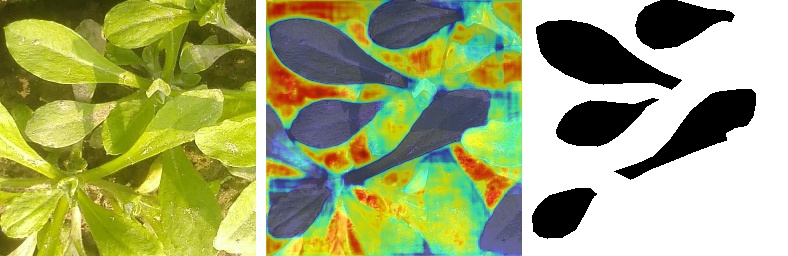
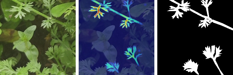
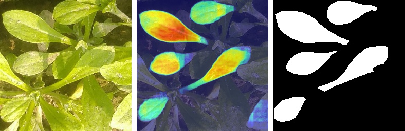
As shown in the examples above, red and yellow regions indicate stronger activation, implying the model’s “attention” for that class. When the highlighted regions align well with the ground truth segmentation mask, it confirms that the model is correctly learning to distinguish between various classes like different weed types or background.

This visualization not only improves transparency but also aids in debugging, trust-building, and model refinement — especially in real-world applications where the consequences of model predictions are significant.

Layer Selection Tips

Want to explore different abstraction levels? Try:

• e1.conv.conv.5: Early encoder layers (low-level features)
• e4.conv.conv.5: Deeper encoder layers
• b.conv.5: Bottleneck
• d4.conv.conv.5: Final decoder layers (good for attention visualization)

Conclusion

In this post, we implemented GradCAM to visualize per-class attention maps for a multiclass segmentation model in PyTorch. By overlaying these maps on the original input, we gained deeper insights into what the model “sees” while making predictions.

You learned:

• What is GradCAM, and why does it matter
• How to compute and overlay class-specific heatmaps
• How to debug and interpret your segmentation models

If you found this helpful, consider starring the GitHub repo or sharing it with others working in computer vision!

Code: Multiclass Segmentation in PyTorch

Next Steps

• Try GradCAM++ for sharper maps.
• Use Guided Backpropagation for higher resolution.
• Integrate into your model monitoring or validation pipeline.