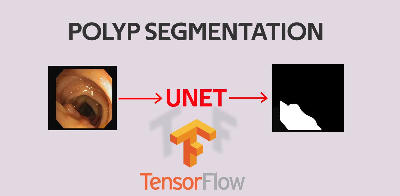
In this tutorial, we will learn about how to perform polyp segmentation using deep learning, UNet architecture, OpenCV, and other libraries. We will use a polyp segmentation dataset to understand how semantic segmentation is applied to real-world data.
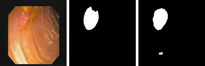
In polyp segmentation, the images with polyp are given to a trained model and it will give us a binary image or mask. This binary image consists of black and white pixels, where white denotes the polyp in image and black denotes the background.
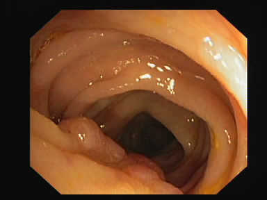
Image with polyp 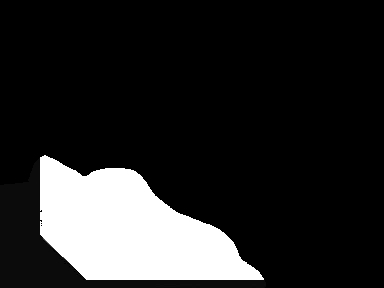
Binary mask
Deep learning is a powerful way to perform computer vision tasks. The main advantage of this approach is the ability to achieve unprecedented accuracy in many computer vision tasks like object detection, semantic segmentation, face detection, etc.
What is Semantic Segmentation
Semantic segmentation is one of the challenges in computer vision research. It can be thought of as a classification problem, but at the pixel level because you need to predict the label or class of every pixel in an image.
Semantic segmentation is a task that steps toward the complete scene understanding by learning to predict what is in the image. The importance of scene understanding lies in its applications to the field of computer vision, such as self-driving vehicles, human-computer interaction, autonomous robots, augmented reality, facial- recognition systems, etc.
Read more:
What is UNet
The UNet is a fully convolutional neural network that was developed by Olaf Ronneberger at the Computer Science Department of the University of Freiburg, Germany. It was especially developed for biomedical image segmentation.
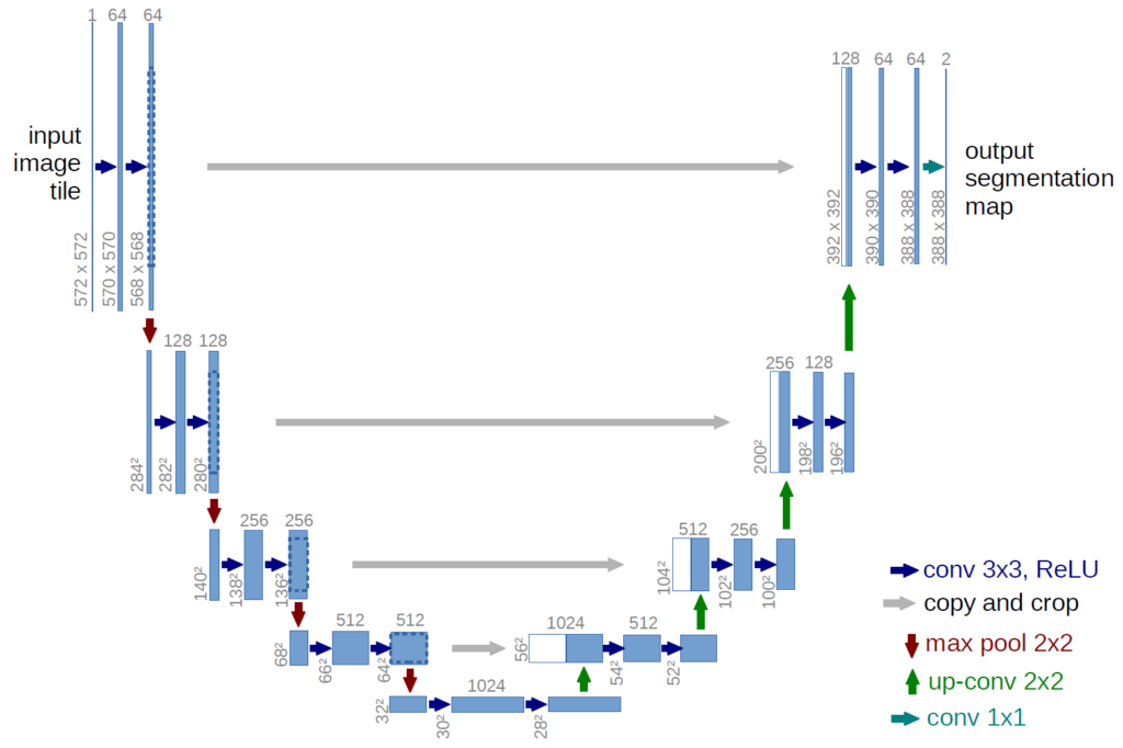
The UNet follows a symmetric architecture shaped like the English letter “U”. It is an improvement over the Fully convolutional networks for semantic segmentation by Evan Shelhamer, Jonathan Long, Trevor Darrell.
Read more about UNet:
Project Structure
In this part of the blog post, let us take a look at the project structure and see what each file and folder represent in the project.
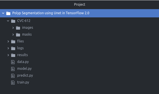
The project has four folders:
- CVC-612/: It consists of the dataset that we are going to use for this project. It contains two sub-folder: images and masks. As their name suggests, these sub-folder contain the images and masks.
- files/: This folder is used to store the CSV file which contains all the information while the model is training. It also stores the model weight file.
- logs/: it contains the TensorBoard log files.
- results/: It is used to store the results after we make predictions on the test dataset.
The project also has four python scripts:
- data.py: This file contains the code for loading the dataset, reading the images and masks. It is also used for creating a tf.data pipeline for training, validation and testing dataset.
- model.py: This file has the code for the UNet architecture which is to segment the polyp images.
- train.py: This file helps the model to train on the training dataset. It is also used save the model which is later used to make predictions on the test dataset.
- predict.py: After the training is finished, this file is used to make predictions on the test dataset.
Understanding the dataset
The dataset contains the image extracted from the colonoscopy videos. These image contains different types polyps. The dataset also include the ground-truth for those images.
You can download the dataset from here or from directly from the Dropbox.
Implementation
Now, we are going to move towards the implementation of the polyp segmentation. For this, I have used TensorFlow 2.0 with Python3.7 in Ubuntu 19.10.
Here, we are going to discuss the different files we are using in the polyp segmentation project.
DATA.PY
The file helps deals with the dataset we’ll be working on. It helps deals with the following tasks:
- It loads the dataset and then split it into training, validation and testing dataset.
- Read the images and masks.
- Building the tf.data pipeline for training, validation and testing dataset.
import os
import numpy as np
import cv2
from glob import glob
import tensorflow as tf
from sklearn.model_selection import train_test_split
At the begriming of the file, we import all the required libraries which include NumPy, Open CV, TensorFlow and others. It also import the function train_test_split, which we are going to use to split the dataset.
def load_data(path, split=0.1):
    images = sorted(glob(os.path.join(path, "images/*")))
    masks = sorted(glob(os.path.join(path, "masks/*")))

    total_size = len(images)
    valid_size = int(split * total_size)
    test_size = int(split * total_size)

    train_x, valid_x = train_test_split(images, test_size=valid_size, random_state=42)
    train_y, valid_y = train_test_split(masks, test_size=valid_size, random_state=42)

    train_x, test_x = train_test_split(train_x, test_size=test_size, random_state=42)
    train_y, test_y = train_test_split(train_y, test_size=test_size, random_state=42)

    return (train_x, train_y), (valid_x, valid_y), (test_x, test_y)
The load_data function loads the CVC-ClinicDB (CVC-612) dataset and returns the training, validation and testing dataset. It takes the dataset path and the dataset split value as the argument.
Let us go ahead an load all the images and masks from their respective directories. Now we use sorted() function to sort images and masks. The images and masks list contains complete paths of the original dataset images and masks.
Now we calculate the size of dataset used for validation and testing purpose. Now we use the train_test_split function to split or divide the polyp dataset into the training, validation and testing. The dataset split ratio is 80:10:10.
def read_image(path):
     path = path.decode()
     x = cv2.imread(path, cv2.IMREAD_COLOR)
     x = cv2.resize(x, (256, 256))
     x = x/255.0
     return x
The read_image function take the image path, load the RGB image as a numpy array, which is resize to 256 x 256 pixels. After that, we normalize the numpy array i.e., divide the numpy array by 255.0.
def read_mask(path):
     path = path.decode()
     x = cv2.imread(path, cv2.IMREAD_GRAYSCALE)
     x = cv2.resize(x, (256, 256))
     x = x/255.0
     x = np.expand_dims(x, axis=-1)
     return x
The read_mask function is same as the read_image except it read the image in grayscale format. At the end of the function, we expand the dimension of the numpy array.
def tf_parse(x, y):
    def _parse(x, y):
        x = read_image(x)
        y = read_mask(y)
        return x, y

    x, y = tf.numpy_function(_parse, [x, y], [tf.float64, tf.float64])
    x.set_shape([256, 256, 3])
    y.set_shape([256, 256, 1])
    return x, y

def tf_dataset(x, y, batch=8):
    dataset = tf.data.Dataset.from_tensor_slices((x, y))
    dataset = dataset.map(tf_parse)
    dataset = dataset.batch(batch)
    dataset = dataset.repeat()
    return dataset
The above two functions tf_parse and tf_dataset are used to build the dataset pipeline.
The tf_dataset function create a tf.data pipeline which takes a list of images, masks paths and the batch size. The tf_parse function parses a single image and mask path.
MODEL.PY
The model.py file contains the code for the Unet architecture which is going to be trained on the polyp segmentation dataset.
import tensorflow as tf
from tensorflow.keras.layers import *
from tensorflow.keras.models import Model
Here, we import all the required libraries.
def conv_block(x, num_filters):
    x = Conv2D(num_filters, (3, 3), padding="same")(x)
    x = BatchNormalization()(x)
    x = Activation("relu")(x)

    x = Conv2D(num_filters, (3, 3), padding="same")(x)
    x = BatchNormalization()(x)
    x = Activation("relu")(x)

    return x
The conv_block is the core of the UNet architecture which consists of two 3×3 convolutions, each with their own batch normalization and a ReLU (Rectified Linear Unit) activation. All the convolution layers in this function use the same number of filters.
def build_model():
    size = 256
    num_filters = [16, 32, 48, 64]
    inputs = Input((size, size, 3))

    skip_x = []
    x = inputs

    ## Encoder
    for f in num_filters:
        x = conv_block(x, f)
        skip_x.append(x)
        x = MaxPool2D((2, 2))(x)

    ## Bridge
    x = conv_block(x, num_filters[-1])

    num_filters.reverse()
    skip_x.reverse()

    ## Decoder
    for i, f in enumerate(num_filters):
        x = UpSampling2D((2, 2))(x)
        xs = skip_x[i]
        x = Concatenate()([x, xs])
        x = conv_block(x, f)

    ## Output
    x = Conv2D(1, (1, 1), padding="same")(x)
    x = Activation("sigmoid")(x)

    return Model(inputs, x)
The build_model function is used to build the entire UNet architecture with the helps of TensorFlow library.
The input size (image size) is 256 pixels and the number of filters are [16, 32, 48, 64]. You can change the input size or number of filters as per your requirement.
We initialized an empty list variable named skip_x which is used to store the skip connection feature maps from the encoder.
Now we build the encoder by looping over the number of filters with the help of the conv_block function. The output of the conv_block is appended to the skip_x, which is going to be used in the decoder part.
After encoder the bridge comes into the play which uses a single conv_block. It helps to connect the encoder and the decoder.
Now, we reverse the num_filters and skip_x list as it will easy the process of information extraction in the decoder block.
Let’s now move on the decoder part of the UNet architecture, and we’ll see how it works. The main purpose of the decoder is to generate the desired semantic segmentation map.
The decoder performs a looping over the number of filters. Inside the loop, a 2×2 upsampling layer is applied. Now the output of the upsamping layers is concatenated with the skip connection from the skip_x list. At last a single conv_block is used to generate the output.
After the decoder part is complete, a 1×1 convolution with the sigmoid activation function is applied. This gives the final output in the form of a binary mask.
TRAIN.PY
The UNet architecture is complete, now the training can of the model can be started. Let’s now understand how UNet architecture is trained on the polyp segmentation dataset.
import os
import numpy as np
import cv2
from glob import glob
import tensorflow as tf
from tensorflow.keras.callbacks import EarlyStopping, ModelCheckpoint, ReduceLROnPlateau, CSVLogger, TensorBoard
from data import load_data, tf_dataset
from model import build_model
All the required functions are imported from the required libraries.
def iou(y_true, y_pred):
     def f(y_true, y_pred):
         intersection = (y_true * y_pred).sum()
         union = y_true.sum() + y_pred.sum() - intersection
         x = (intersection + 1e-15) / (union + 1e-15)
         x = x.astype(np.float32)
         return x
     return tf.numpy_function(f, [y_true, y_pred], tf.float32)
The iou function calculate the Intersection Over Union (IOU) between the ground truth (y_true) and the predicted output (y_pred). This function returns a value between 0 and 1.
if __name__ == "__main__":
     ## Dataset
     path = "CVC-612/"
     (train_x, train_y), (valid_x, valid_y), (test_x, test_y) = load_data(path)
Here the training, validation and testing dataset using the load_data function.
    ## Hyperparameters
    batch = 8
    lr = 1e-4
    epochs = 20
The hyper parameters are defined above which are used while training the UNet architecture.
      train_dataset = tf_dataset(train_x, train_y, batch=batch)
      valid_dataset = tf_dataset(valid_x, valid_y, batch=batch)
The training and validation input dataset pipelines are build with the tf_dataset function. The tf_dataset take the images paths and masks paths as a list. It also takes the batch size.
    model = build_model()

    opt = tf.keras.optimizers.Adam(lr)
    metrics = ["acc", tf.keras.metrics.Recall(), tf.keras.metrics.Precision(), iou]
    model.compile(loss="binary_crossentropy", optimizer=opt, metrics=metrics)
The UNet architecture is defined and built using the build_model function. The Adam optimizer is used with a learning rate value to optimize the architecture. To measure the performance of the architecture four metrics are used:
- Accuracy
- Recall
- Precision
- IOU
     callbacks = [
          ModelCheckpoint("files/model.h5"),
          ReduceLROnPlateau(monitor='val_loss', factor=0.1, patience=4),
          CSVLogger("files/data.csv"),
          TensorBoard(),
          EarlyStopping(monitor='val_loss', patience=10, restore_best_weights=False)
     ]
The following callbacks are used:
- ModelCheckpoint: Save the model weight file after every epoch.
- ReduceLROnPlateau: Reduce learning rate when a metric has stopped improving.
- CSVLogger: Save all the training data in a CSV file.
- TensorBoard: Helps you to visualize the data.
- EarlyStopping: Stop training when a monitored quantity has stopped improving.
    train_steps = len(train_x)//batch
    valid_steps = len(valid_x)//batch

    if len(train_x) % batch != 0:
        train_steps += 1
    if len(valid_x) % batch != 0:
        valid_steps += 1

    model.fit(train_dataset,
        validation_data=valid_dataset,
        epochs=epochs,
        steps_per_epoch=train_steps,
        validation_steps=valid_steps,
        callbacks=callbacks)
First we define the training and validation steps, which define the number of batches in an epoch. The fit function starts training the model which is define using the build_model function.
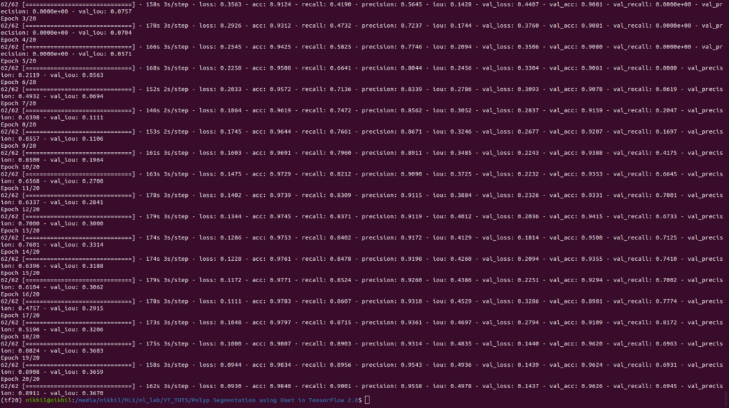
I trained the model on 20 epoch and the final epoch value in the table given below.
| METRICS | VALUE |
| Loss | 0.0930 |
| Accuracy | 0.9840 |
| Recall | 0.9001 |
| Precision | 0.9558 |
| IoU | 0.4978 |
| Validation Loss | 0.1437 |
| Validation Accuracy | 0.9636 |
| Validation Recall | 0.6945 |
| Validation Precision | 0.8911 |
| Validation IoU | 0.3670 |
PREDICT.PY
The predict.py file is used to evaluate the test dataset and also used to save the predicted mask.
import os
import numpy as np
import cv2
import tensorflow as tf
from tensorflow.keras.utils import CustomObjectScope
from tqdm import tqdm
from data import load_data, tf_dataset
from train import iou
Again importing the required libraries and the files.
def read_image(path):
     x = cv2.imread(path, cv2.IMREAD_COLOR)
     x = cv2.resize(x, (256, 256))
     x = x/255.0
     return x

 def read_mask(path):
     x = cv2.imread(path, cv2.IMREAD_GRAYSCALE)
     x = cv2.resize(x, (256, 256))
     x = np.expand_dims(x, axis=-1)
     return x
The read_image and read_mask functions are used to read the image and mask respectively. In the read_image function, the image is normalized, as the image need to be feed into the trained Unet architecture for prediction.
def mask_parse(mask):
     mask = np.squeeze(mask)
     mask = [mask, mask, mask]
     mask = np.transpose(mask, (1, 2, 0))
     return mask
The mask_parse function is used while joining the input image, ground truth mask and the predicted mask to form a single image.
if __name__ == "__main__":
     ## Dataset
     path = "CVC-612/"
     batch_size = 16
     (train_x, train_y), (valid_x, valid_y), (test_x, test_y) = load_data(path)
The training, validation and test data is loaded using the load_data function, but we will only use the test data only. Thebatch size 16 is also defined for the evaluation.
     test_dataset = tf_dataset(test_x, test_y, batch=batch_size)

     test_steps = (len(test_x)//batch_size)
     if len(test_x) % batch_size != 0:
         test_steps += 1
The test dataset pipeline is build and the test steps are defined.
     with CustomObjectScope({'iou': iou}):
         model = tf.keras.models.load_model("files/model.h5")
The trained Unet architecture is loaded and defined in the model variable.
model.evaluate(test_dataset, steps=test_steps)
Now we start the evaluation of the test dataset to each is performance. The value of loss and different metrics is in the table given below.
| METRICS | VALUE |
| Loss | 0.449 |
| Accuracy | 0.9624 |
| Recall | 0.7803 |
| Precison | 0.8437 |
| IoU | 0.4184 |
The metrics performance is decent, its not that much. It can be improved by:
- Training on more epoch.
- Applying data augmentation.
- Increasing the number of filters.
- Tuning the hyperparameters.
     for i, (x, y) in tqdm(enumerate(zip(test_x, test_y)), total=len(test_x)):
           x = read_image(x)
           y = read_mask(y)
           y_pred = model.predict(np.expand_dims(x, axis=0))[0] > 0.5
           h, w, _ = x.shape
           white_line = np.ones((h, 10, 3)) * 255.0
           all_images = [
              x * 255.0, white_line,
              mask_parse(y), white_line,
              mask_parse(y_pred) * 255.0
           ]
           image = np.concatenate(all_images, axis=1)
           cv2.imwrite(f"results/{i}.png", image)
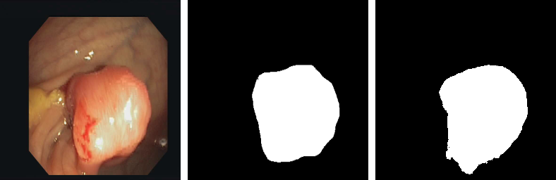
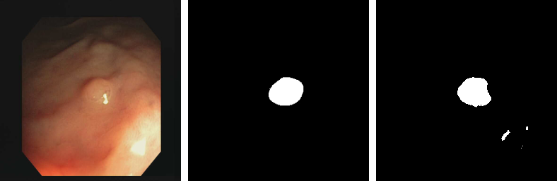
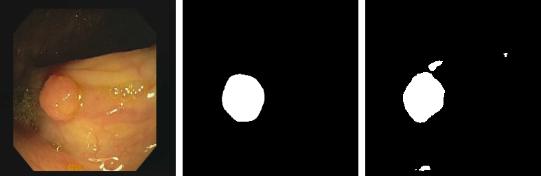
The code given above is used to make generate the predicted mask on the test images. A threshold value of 0.5 is applied on the predicted mask. The input image, ground truth and the predicted mask are joined together to form a single image.
Some of the sample shot of test results are given below.
| INPUT IMAGE | GROUND TRUTH | PREDICTED MASK |
Conclusion
In this tutorial, you have learned to semantic segmentation using UNet architecture using polyp segmentation dataset. If you find this tutorial useful then share it with your friends and signup for more such stuff.

Thanks for great tutorial …
Thank you for sharing!
Your explaintion helps alot, I learned something there.
Great Tutorial as always. I learnt a lot from you, sir. But I got a question. I was implementing lung nodule segmentation and I am stuck on how to incorporate the data augmentation which you suggest would improve the model performance.
Can you please give me a proper hint as to how to go about that. I have tried to read the TensoFlow doc and implemented it, but keep getting errors. I guess inputing the augmentation into the dataset API pipeline was hard for me.
I have some issues reading in the validation steps needs for the final epoch pass in module.fit step. So the missing link can be traced if you share your model layer and parameters summary table that you can easily write out after you get your model compiled. Thanks
Great Work.. Very beneficial to a novice like me. Tried to run the same code on polyp data set itself with valid_split=0.3,test_split=0.1 .and the
Epochs was made 35.These were the only difference which was made in the code . But during prediction phase ,met with an error with the code
with CustomObjectScope({‘iou’: iou}):
model = tf.keras.models.load_model(“files/model.h5″)
model.evaluate(test_dataset,steps=test_steps).
Showing that ” TypeError: ‘<' not supported between instances of 'function' and 'str' …… with the code…." model.evaluate(test_dataset,steps=test_steps)."
Can you please help me to rectify this error….
the size of original image is 384 x 288, why do you resize it to 256 x 256?
I have resized the images to 256 x 256 just for my easiness. You can use the original size also.
Hi Nikhil – This is a very nice post! I have a question, do I absolutely need to use cv2 for the functions executed using cv2 in your scripts shown here (such as imwrite, imread, resize…), or there are other Python alternatives to this? Thanks!!!
if my mask data is RGB how can i implementation this code??
I have a problem, when i cleared file results, and try to start predict.py, only 2 images are displaying in folder. And also, when i am trying to put full database of images and mask, Training going in 20 epoch within only 62 times. Do u have some solutions?
ImportError: cannot import name ‘load_data’ from ‘data’ (C:\Users\Aravinda\anaconda3\lib\site-packages\data\__init__.py)
Hello Nikhil,
Great article and video really informative and very efficient way of implementing data pipeline but when I was trying to implement same for another dataset
Dataset URL: https://www.kaggle.com/datasets/jeetblahiri/bccd-dataset-with-mask
This is the error which I am getting
Epoch 1/20
—————————————————————————
ValueError Traceback (most recent call last)
in ()
—-> 1 model.fit(
2 train_dataset,
3 validation_data = valid_dataset,
4 epochs = epochs,
5 steps_per_epoch = train_steps,
1 frames
/usr/local/lib/python3.10/dist-packages/keras/src/metrics/reduction_metrics.py in reduce_to_samplewise_values(values, sample_weight, reduce_fn, dtype)
39 )
40
—> 41 values_ndim = len(values.shape)
42 if values_ndim > 1:
43 values = reduce_fn(values, axis=list(range(1, values_ndim)))
ValueError: Cannot take the length of shape with unknown rank.
It would be really helpful if you can help me with this and let me know if you need any more information,
Thank you and best regards.