
The article explores the Naive Bayes classifier, its workings, the underlying naive Bayes algorithm, and its application in machine learning. Through an intuitive example and Python implementation, the article demonstrates how Naive Bayes in Python can be applied for real-world classification tasks. Complete with code, evaluation metrics, and practical insights, this guide provides a thorough understanding of the Bayes classifier and its use cases.
What is Naive Bayes
The Naive Bayes classifier is a supervised learning algorithm based on Bayes’ Theorem, which strongly assumes that features are independent. Due to its simplicity and efficiency, the naive Bayes algorithm works particularly well for small datasets and high-dimensional data, making it ideal for applications such as natural language processing, spam detection, and medical diagnosis.
The classifier is called “Naive” because it assumes that all features (attributes) are independent of one another, a condition that rarely holds true in real-world datasets. However, despite this naive assumption, the naive Bayes classifier often delivers highly accurate predictions and performs remarkably well in many classification tasks, even when the independence assumption is violated.
ALSO READ:
- Generative and Discriminative Models in Machine Learning
- Mastering k-Nearest Neighbor Algorithm in R
Bayes’ Theorem
Bayes’ Theorem is a fundamental concept in probability theory that describes how to update the probability of a hypothesis based on new evidence. It provides a way to calculate the posterior probability of an event by combining the prior probability and the likelihood of observing the new data under that event.
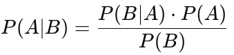
Where:
- P(A∣B): Posterior probability of class A (target) given predictor B (features).
- P(A): Prior probability of class A, the overall likelihood of A happening.
- P(B∣A): Likelihood or the probability of predictor B given that class A has occurred.
- P(B): Prior probability of predictor B, the likelihood of seeing predictor B regardless of the class.
Types of Naive Bayes Classifiers
- Gaussian Naive Bayes: Assumes that the features follow a normal (Gaussian) distribution. This is useful for continuous data.
- Multinomial Naive Bayes: Used for discrete data, such as the occurrence of events (e.g., word counts in text classification).
- Bernoulli Naive Bayes: Designed for binary or Boolean features, particularly effective for binary text classification where words are present or absent in a document.
Bayes Theorem Explanation with an Example
Let’s consider a more intuitive example: We use a simple dataset to classify whether a person buys a product (Yes/No) based on their age and income level.
| Person | Age | Income | Buys Product (Yes/No) |
|---|---|---|---|
| 1 | Young | High | No |
| 2 | Young | Medium | No |
| 3 | Middle | High | Yes |
| 4 | Old | High | Yes |
| 5 | Old | Medium | No |
| 6 | Middle | Low | Yes |
| 7 | Young | Low | No |
| 8 | Old | Low | No |
| 9 | Young | Medium | No |
| 10 | Middle | High | Yes |
Here, we have 10 instances. Our goal is to predict whether a person will buy a product based on age and income.
Let’s say we want to predict a new person with the following characteristics:
- Age: Young
- Income: High
We will use Bayes’ Theorem to calculate the probability of this person buying the product (Yes/No).
Step 1: Calculate the Prior Probability — P(Buys Product)
From the dataset:
P(Yes): Probability of a person buying the product.

P(No): Probability of a person not buying the product.

Step 2: Calculate the Likelihood — P(Age = Young | Buys Product) and P(Income=High | Buys Product)
Next, we calculate the likelihoods based on the conditional probabilities of the features (age and income) for each class (Yes/No).
For Buys Product = Yes:


For Buys Product = No:


Step 3: Apply Bayes’ Theorem
We now apply Bayes’ Theorem to calculate the posterior probabilities — P(Yes | Age = Young, Income = High) and P(No | Age = Young, Income=High)


We don’t need to calculate P(Age=Young, Income=High) explicitly because it is the same for both the “Yes” and “No” cases. So we can compare the numerators directly.
For Yes:


For No:


Step 4: Conclusion


Since P(No) is higher than P(Yes), the Naive Bayes classifier would predict “No” — the person is not likely to buy the product.
Naive Bayes Algorithm
The steps involved in the Naive Bayes algorithm are as follows:
Calculate the prior probability for each class based on the training data.

2. Calculate the likelihood for each feature within a class. For Gaussian Naive Bayes, this is done using the Gaussian (Normal) distribution formula:
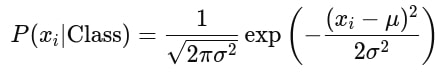
Where:
- xi: Value of the feature.
- μ: Mean of the feature in the class.
- σ2: Variance of the feature in the class.
Apply Bayes’ Theorem to calculate the posterior probability for each class.
Assign the class label with the highest posterior probability to the new instance.
Advantages and Disadvantages of Naive Bayes Classifier
Advantages
- Simplicity: The Naive Bayes classifier is very easy to understand and implement, making it a great starting point for machine learning beginners.
- Speed and Efficiency: It is computationally efficient and works well with small and high-dimensional data. The naive Bayes algorithm performs classification quickly, even on large datasets.
- Handles Missing Data: The model can handle missing data well by ignoring the instance or using probabilities calculated from the available data.
- Performs Well with Categorical Data: Naive Bayes is particularly effective with categorical input data, making it a good choice for text classification tasks like spam detection or sentiment analysis.
- Low Training Time: As it calculates probabilities directly from the training data, the training time for naive Bayes machine learning models is minimal.
- Works Well with High-Dimensional Data: Naive Bayes still performs efficiently in problems with many features (e.g., text classification with thousands of words).
Disadvantages
- Naive Assumption: The naive Bayes classifier’s core assumption—that features are independent— is rarely true in real-world datasets. This can lead to inaccuracies when features are highly correlated.
- Zero-Frequency Problem: If a categorical variable in the test set contains a category that wasn’t present in the training set, naive Bayes assigns a probability of 0, which can negatively affect predictions. This can be resolved by using techniques like Laplace smoothing.
- Not Ideal for Continuous Data: While the Gaussian Naive Bayes variant can handle continuous data, other algorithms like Decision Trees or SVMs may perform better with complex relationships in continuous variables.
- Limited Expressiveness: Due to its simplicity, the naive Bayes classifier may struggle with complex decision boundaries, making it less suited for certain types of tasks where other models, like neural networks, would be more appropriate.
- Over-sensitivity to Imbalanced Data: Naive Bayes can be biased towards the majority class if the data is imbalanced, especially when dealing with highly skewed datasets.
Despite these disadvantages, Naive Bayes in Python is an excellent tool for quick and efficient classification, especially in cases where the independence assumption approximately holds or when simplicity and speed are prioritized.
Python Implementation with Iris Dataset
Step 1: Importing Libraries and Loading Data
import numpy as np
import pandas as pd
import seaborn as sns
from sklearn.datasets import load_iris
from sklearn.model_selection import train_test_split
from sklearn.naive_bayes import GaussianNB
from sklearn.metrics import accuracy_score, confusion_matrix, classification_report
import matplotlib.pyplot as plt

# Load the Iris dataset
iris = load_iris()
X = iris.data
y = iris.target

# Splitting the dataset into training and test sets
X_train, X_test, y_train, y_test = train_test_split(X, y, test_size=0.3, random_state=42)
Dataset Description: The Iris dataset has 150 samples with four features: sepal length, sepal width, petal length, and petal width. The target variable is the iris species: Setosa, Versicolour, and Virginica.
Step 2: Training the Naive Bayes Classifier
# Initialize the Gaussian Naive Bayes model
gnb = GaussianNB()

# Fit the model on the training data
gnb.fit(X_train, y_train)

# Predicting the labels on the test set
y_pred = gnb.predict(X_test)
Step 3: Evaluating the Model
# Calculate the accuracy of the model
accuracy = accuracy_score(y_test, y_pred)
print(f'Accuracy: {accuracy:.2f}')

# Confusion Matrix
conf_matrix = confusion_matrix(y_test, y_pred)
print(f'Confusion Matrix:\n{conf_matrix}')

# Classification Report
class_report = classification_report(y_test, y_pred, target_names=iris.target_names)
print(f'Classification Report:\n{class_report}')
Output
Accuracy: 0.98
Confusion Matrix:
[[19  0  0]
 [ 0 12  1]
 [ 0  0 13]]
Classification Report:
              precision    recall  f1-score   support

      setosa       1.00      1.00      1.00        19
  versicolor       1.00      0.92      0.96        13
   virginica       0.93      1.00      0.96        13

    accuracy                           0.98        45
   macro avg       0.98      0.97      0.97        45
weighted avg       0.98      0.98      0.98        45
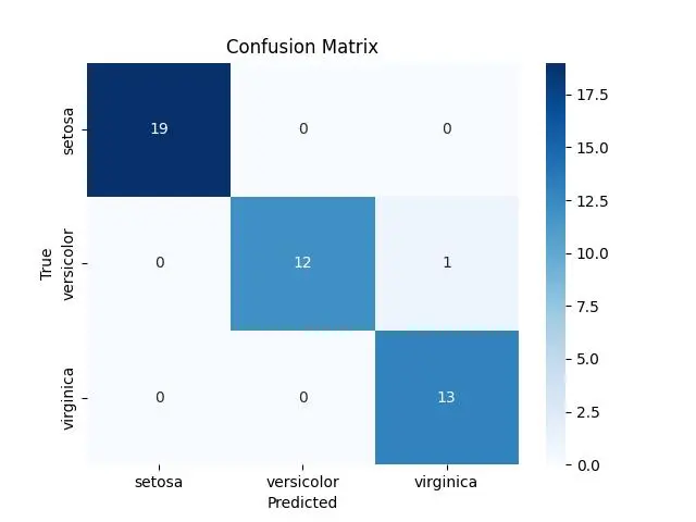
Step 4: Visualizing Results
sns.heatmap(conf_matrix, annot=True, cmap="Blues", fmt="g", xticklabels=iris.target_names, yticklabels=iris.target_names)
plt.title('Confusion Matrix')
plt.xlabel('Predicted')
plt.ylabel('True')
plt.show()
Conclusion
The Naive Bayes classifier is a lightweight yet highly effective algorithm for classification tasks. Its simplicity, speed, and accuracy make it a go-to choice in many machine-learning applications. Implementing the Naive Bayes classifier in Python using libraries like scikit-learn enables developers to easily harness its power for real-world problems. The naive Bayes classifier provides an efficient solution with minimal computational overhead for text classification or other machine-learning tasks. This versatility extends the use of naive Bayes in machine learning to many practical scenarios.