TensorFlow is a powerful library for machine learning that allows for the easy implementation of various algorithms, including linear regression. In this tutorial, we will be using TensorFlow tape gradient to implement a linear regression model and plot the loss graph and x and y on matplotlib.
First, we will start by importing the necessary libraries:
import tensorflow as tf
import matplotlib.pyplot as plt
Next, we will generate some fake data for our linear regression model. We will use the tf.random.normal() function to generate random x and y values, and we will use a slope of 2 and an intercept of 1 to generate our y values.
# Generate fake data
num_samples = 1000
x = tf.random.normal([num_samples])
y = 2 * x + 1 + tf.random.normal([num_samples])
Now, we will define our model using the tf.keras.Sequential() function and add a single layer with one input and one output.
# Define model
model = tf.keras.Sequential([
    tf.keras.layers.Dense(1, input_shape=(1,))
])
Next, we will define our loss function and optimizer. We will use the mean squared error loss function and the Adam optimizer.
# Define loss and optimizer
loss_fn = tf.keras.losses.MeanSquaredError()
optimizer = tf.keras.optimizers.Adam()
Now, we will use the TensorFlow tape gradient method to train our model. We will loop through the data for a specified number of iterations and update the model’s weights using the optimizer.
# Train model
num_epochs = 1000
loss_values = []
for epoch in range(num_epochs):
    with tf.GradientTape() as tape:
        y_pred = model(x)
        loss = loss_fn(y, y_pred)
        loss_values.append(loss.numpy())
    grads = tape.gradient(loss, model.trainable_variables)
    optimizer.apply_gradients(zip(grads, model.trainable_variables))
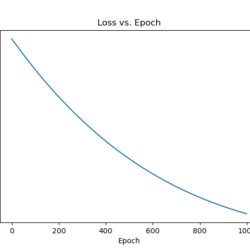
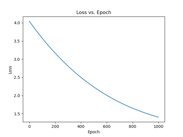
Finally, we will plot the loss graph and x and y on matplotlib.
# Plot loss graph
plt.plot(loss)
plt.title('Loss vs. Epoch')
plt.xlabel('Epoch')
plt.ylabel('Loss')
plt.show()
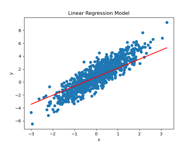
# Plot x and y
plt.scatter(x, y)
plt.plot(x, model(x), 'r')
plt.title('Linear Regression Model')
plt.xlabel('x')
plt.ylabel('y')
plt.show()
And that’s it! We have successfully implemented a linear regression model using TensorFlow tape gradient and plotted the loss graph and x and y on matplotlib. You can experiment with different values for the number of samples, slope, and intercept to see how it affects the model’s performance. Happy coding!