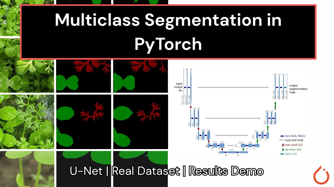
Multiclass Segmentation in PyTorch using U-Net

Semantic segmentation is a crucial task in computer vision that involves labeling each pixel in an image with its corresponding class. In this blog post, we’ll dive into building a multiclass semantic segmentation pipeline using the U-Net architecture with PyTorch. Our goal is to segment different types of weeds from agricultural images — a use case highly relevant to precision farming.

What is Multiclass Segmentation?

Multiclass segmentation assigns each pixel in an image to one of several classes. Unlike binary segmentation (foreground vs. background), multiclass segmentation deals with more than two semantic categories.

The images and RGB masks from the Weed Segmentation dataset

In our case, the categories are:

Background
Weed type 1
Weed type 2

Project Structure

Multiclass-Segmentation-in-PyTorch
├── files/             # Stores checkpoint and score metrics
├── results/           # Saved predictions 
├── Weeds-Dataset/     # Dataset directory
├── model.py           # U-Net model
├── utils.py           # Utility functions
├── metrics.py         # Loss functions
├── train.py           # Training script
├── test.py            # Evaluation script

Dataset

We use a custom dataset located in Weeds-Dataset/weed_augmented. It contains two subfolders:

images/: RGB images (.jpg)
masks/: Segmentation masks (.png), where different colors represent different classes.

The dataset can be downloaded from here: Multiclass Weed Dataset

Class Color Mapping:

Background: [0, 0, 0]
Weed-1: [0, 0, 128]
Weed-2: [0, 128, 0]

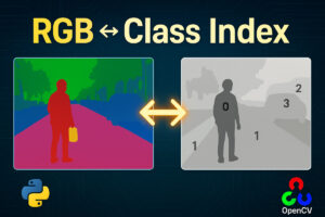
The color-coded masks are converted to class indices internally before training.

ALSO READ:

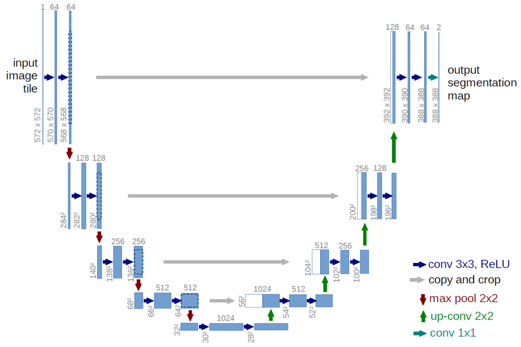
Model: U-Net Architecture

The U-Net model is built from scratch in model.py using PyTorch’s nn.Module. The architecture follows the classic encoder–bottleneck–decoder format. Let’s break it down step-by-step.

The block diagram of original UNet Architecture

Imports

import torch
import torch.nn as nn

We use PyTorch’s core modules for building neural network layers (nn.Module, Conv2d, BatchNorm2d, ReLU, etc.).

Convolutional Blocks

The conv_block is the basic building block. This block applies two convolutional layers, followed by BatchNorm and ReLU activations:

class conv_block(nn.Module):
    def __init__(self, in_c, out_c):
        super().__init__()
        self.conv = nn.Sequential(
            nn.Conv2d(in_c, out_c, kernel_size=3, padding=1),
            nn.BatchNorm2d(out_c),
            nn.ReLU(inplace=True),
            nn.Conv2d(out_c, out_c, kernel_size=3, padding=1),
            nn.BatchNorm2d(out_c),
            nn.ReLU(inplace=True)
        )

    def forward(self, inputs):
        return self.conv(inputs)

Arguments:

in_c: Number of input channels
out_c: Number of output channels

This block helps extract high-level spatial features while maintaining spatial resolution using the same padding (padding=1).

Encoder Block: Downsampling

Each encoder block applies a conv_block followed by MaxPooling to reduce spatial dimensions:

class encoder_block(nn.Module):
    def __init__(self, in_c, out_c):
        super().__init__()
        self.conv = conv_block(in_c, out_c)
        self.pool = nn.MaxPool2d((2, 2))

    def forward(self, inputs):
        x = self.conv(inputs)
        p = self.pool(x)
        return x, p

Returns:

x: Feature map before pooling (used in skip connection)
p: Pooled feature map passed to the next encoder

Decoder Blocks: Upsampling + Skip Connection

Each decoder block upsamples the input, concatenates it with the corresponding encoder output (skip connection), and applies a convolution block:

class decoder_block(nn.Module):
    def __init__(self, in_c, out_c):
        super().__init__()
        self.up = nn.ConvTranspose2d(in_c, out_c, kernel_size=2, stride=2, padding=0)
        self.conv = conv_block(out_c + out_c, out_c)

    def forward(self, inputs, skip):
        x = self.up(inputs)
        x = torch.cat([x, skip], axis=1)
        x = self.conv(x)
        return x

Key operations:

ConvTranspose2d: Upsamples the feature map
torch.cat: Concatenates skip connection along the channel axis

U-Net Model

This is the full U-Net model that connects the encoder, bottleneck, and decoder:

class build_unet(nn.Module):
    def __init__(self, num_classes=3):
        super().__init__()

        # Encoder
        self.e1 = encoder_block(3, 64)
        self.e2 = encoder_block(64, 128)
        self.e3 = encoder_block(128, 256)
        self.e4 = encoder_block(256, 512)

        # Bottleneck
        self.b = conv_block(512, 1024)

        # Decoder
        self.d1 = decoder_block(1024, 512)
        self.d2 = decoder_block(512, 256)
        self.d3 = decoder_block(256, 128)
        self.d4 = decoder_block(128, 64)

        # Output Layer
        self.outputs = nn.Conv2d(64, num_classes, kernel_size=1, padding=0)

    def forward(self, inputs):
        s1, p1 = self.e1(inputs)
        s2, p2 = self.e2(p1)
        s3, p3 = self.e3(p2)
        s4, p4 = self.e4(p3)

        b = self.b(p4)

        d1 = self.d1(b, s4)
        d2 = self.d2(d1, s3)
        d3 = self.d3(d2, s2)
        d4 = self.d4(d3, s1)

        outputs = self.outputs(d4)
        return outputs

Explanation:

Input goes through 4 encoder blocks → bottleneck → 4 decoder blocks
Skip connections ensure the decoder retains spatial details
Final Conv2d projects the decoder output to num_classes logits for each pixel

Utility Functions

The utils.py script is a helper module containing reusable functions and classes to support training, checkpointing, reproducibility, and more. These utilities improve code organization, readability, and modularity.

Imports:

import os
import random
import numpy as np
import torch
from sklearn.utils import shuffle

os, random: For file/directory management and seeding randomness
numpy: Array manipulations
torch: Deep learning operations
shuffle: Maintains order when shuffling datasets

Seeding:

def seeding(seed):
    random.seed(seed)
    os.environ["PYTHONHASHSEED"] = str(seed)
    np.random.seed(seed)
    torch.manual_seed(seed)
    torch.cuda.manual_seed(seed)
    torch.backends.cudnn.deterministic = True

This function ensures reproducibility by seeding all random number generators across Python, NumPy, and PyTorch. Also sets torch.backends.cudnn.deterministic = True to make CUDA operations deterministic.

Use this at the start of any training or testing script.

Create Directory:

def create_dir(path):
    if not os.path.exists(path):
        os.makedirs(path)

Creates a directory if it doesn’t already exist. Ensures that logs, checkpoints, or result folders are properly generated.

Shuffling:

def shuffling(x, y):
    x, y = shuffle(x, y, random_state=42)
    return x, y

Takes two arrays (e.g., image and mask paths) and returns shuffled versions of both, ensuring correspondence between image and mask is preserved.

Epoch Time Calculation:

def epoch_time(start_time, end_time):
    elapsed_time = end_time - start_time
    elapsed_mins = int(elapsed_time / 60)
    elapsed_secs = int(elapsed_time - (elapsed_mins * 60))
    return elapsed_mins, elapsed_secs

Returns training time in a human-readable format: minutes and seconds.

Save Checkpoint:

def save_checkpoint(model, optimizer, epoch, loss, checkpoint_path):
    torch.save({
        'epoch': epoch,
        'model_state_dict': model.state_dict(),
        'optimizer_state_dict': optimizer.state_dict(),
        'loss': loss,
    }, checkpoint_path)
    print(f"Checkpoint saved at epoch {epoch}")

Saves the model state and optimizer state into a .pth file. This allows training to be resumed later.

Load Checkpoint:

def load_checkpoint(model, optimizer, checkpoint_path):
    if os.path.exists(checkpoint_path):
        checkpoint = torch.load(checkpoint_path)
        model.load_state_dict(checkpoint['model_state_dict'])
        optimizer.load_state_dict(checkpoint['optimizer_state_dict'])
        epoch = checkpoint['epoch']
        print(f"Checkpoint loaded from epoch {epoch}")
        return model, optimizer, epoch
    else:
        print("No checkpoint found, starting from scratch.")
        return model, optimizer, 0

Loads model and optimizer states from a checkpoint file. Returns the epoch number for resuming training.

Early Stopping:

class EarlyStopping:
    def __init__(self, patience=5, verbose=False, delta=0):
        self.patience = patience
        self.verbose = verbose
        self.delta = delta
        self.counter = 0
        self.best_loss = float('inf')
        self.early_stop = False

    def __call__(self, val_loss, model, optimizer, epoch, checkpoint_path):
        if self.best_loss - val_loss > self.delta:
            self.best_loss = val_loss
            self.counter = 0
            save_checkpoint(model, optimizer, epoch, val_loss, checkpoint_path)

        else:
            self.counter += 1
            if self.verbose:
                print(f"EarlyStopping counter: {self.counter} of {self.patience}")
            if self.counter >= self.patience:
                self.early_stop = True
                print("Early stopping triggered")

A custom class that monitors validation loss and stops training early if there’s no improvement after a defined number of epochs (patience).

How it works:

An improvement in validation loss saves the model.
Otherwise, increments a counter.
Once the counter reaches patience, it sets early_stop = True.

Loss Functions

In semantic segmentation, choosing the right loss function is crucial — especially in multiclass settings or when classes are imbalanced. The metrics.py file defines two custom loss functions:

DiceLoss: For measuring the overlap between predicted and ground truth masks.
DiceCELoss: A combination of Dice Loss and Cross Entropy Loss for more robust optimization.

Imports:

import torch
import torch.nn as nn
import torch.nn.functional as F

torch.nn: Required to define loss functions as PyTorch modules
F.softmax, F.one_hot: Used for normalizing outputs and handling target labels

Dice Loss

The Dice coefficient measures the overlap between two samples. It ranges from 0 (no overlap) to 1 (perfect overlap). Dice Loss is defined as:

class DiceLoss(nn.Module):
    def __init__(self, num_classes, smooth=1e-5, ignore_index=None):
        super(DiceLoss, self).__init__()
        self.num_classes = num_classes
        self.smooth = smooth
        self.ignore_index = ignore_index

    def forward(self, logits, targets):
        """
        logits: [B, C, H, W] (raw outputs from model)
        targets: [B, H, W] (ground truth class indices)
        """
        probs = F.softmax(logits, dim=1)  # [B, C, H, W]
        targets_one_hot = F.one_hot(targets, num_classes=self.num_classes).permute(0, 3, 1, 2).float()

        if self.ignore_index is not None:
            mask = (targets != self.ignore_index).unsqueeze(1)  # [B, 1, H, W]
            probs = probs * mask
            targets_one_hot = targets_one_hot * mask

        intersection = torch.sum(probs * targets_one_hot, dim=(0, 2, 3))
        union = torch.sum(probs + targets_one_hot, dim=(0, 2, 3))

        dice = (2 * intersection + self.smooth) / (union + self.smooth)
        return 1.0 - dice.mean()

Arguments:

num_classes: Total number of segmentation classes.
smooth: A small value to prevent division by zero.
ignore_index: If provided, skips that class when computing loss (useful for unlabeled areas).

Forward Method:

logits: Raw output from the model, shape [B, C, H, W]
targets: Ground truth class indices, shape [B, H, W]

It’s Working:

Apply softmax to convert logits to probabilities.
Convert target labels to one-hot encoding.
Optionally apply a mask to ignore certain indices.
Compute the intersection and union.
Return 1 - Dice coefficient.

Dice + CrossEntropy Loss

Combines Dice Loss and Cross Entropy Loss into a single objective:

class DiceCELoss(nn.Module):
    def __init__(self, num_classes, weight=None, dice_weight=1.0, ce_weight=1.0, ignore_index=None):
        super(DiceCELoss, self).__init__()
        self.dice = DiceLoss(num_classes=num_classes, ignore_index=ignore_index)
        self.ce = nn.CrossEntropyLoss(weight=weight, ignore_index=ignore_index)
        self.dice_weight = dice_weight
        self.ce_weight = ce_weight

    def forward(self, logits, targets):
        loss_dice = self.dice(logits, targets)
        loss_ce = self.ce(logits, targets)
        return self.dice_weight * loss_dice + self.ce_weight * loss_ce

Arguments:

num_classes: Number of segmentation classes
weight: Class-wise weights (optional)
dice_weight: Multiplier for Dice loss
ce_weight: Multiplier for Cross Entropy loss
ignore_index: Skip this class while computing loss

Why Use Dice + Cross Entropy?

Loss Type	Benefit
Cross Entropy	Penalizes incorrect class predictions
Dice Loss	Focuses on pixel overlap
Combined Loss	Best of both worlds

This is especially important when some classes are underrepresented (e.g., small weeds vs large background areas).

Training Pipeline

The train.py script orchestrates the training and validation loop for our U-Net model. It includes:

Data loading and splitting
Augmentation strategies
Model training and evaluation
Checkpointing and early stopping

Let’s break it down step by step.

Imports

We import the required libraries:

import os, random, time, datetime
import numpy as np, pandas as pd
import albumentations as A
import cv2
from PIL import Image
from glob import glob
from tqdm import tqdm
import torch
import torch.nn as nn
from torch.utils.data import Dataset, DataLoader
from torchvision import transforms
from sklearn.model_selection import train_test_split

We also import custom modules:

from utils import seeding, create_dir, shuffling, epoch_time, EarlyStopping, save_checkpoint, load_checkpoint
from metrics import DiceLoss, DiceCELoss
from model import build_unet

Loading Dataset

def load_data(dataset_path, split=0.2):
   images = sorted(glob(os.path.join(dataset_path, "images", "*.jpg")))
   masks = sorted(glob(os.path.join(dataset_path, "masks", "*.png")))
   assert len(images) == len(masks)

   split_num = int(split * len(images))
   train_x, valid_x, train_y, valid_y = train_test_split(images, masks, test_size=split_num, random_state=42)
   train_x, test_x, train_y, test_y = train_test_split(train_x, train_y, test_size=split_num, random_state=42)

   return (train_x, train_y), (valid_x, valid_y), (test_x, test_y)

This function loads image and mask paths, then splits them into train, validation, and test sets using train_test_split().

split: Fraction for validation/test (default: 20% of dataset)
Returns: train_x, train_y, valid_x, valid_y, test_x, test_y

So, we use 60% of the data for training, and the remaining 40% data is split equally between the validation and testing datasets.

Dataset Class

This is a custom PyTorch Dataset for loading and preprocessing image-mask pairs.

class DATASET(Dataset):
    def __init__(self, images_path, masks_path, size, colormap, transform=None):
        super().__init__()

        self.images_path = images_path
        self.masks_path = masks_path
        self.size = size
        self.colormap = colormap
        self.transform = transform
        self.n_samples = len(images_path)

    def __getitem__(self, index):
        """ Image """
        image = cv2.imread(self.images_path[index], cv2.IMREAD_COLOR)
        mask = cv2.imread(self.masks_path[index], cv2.IMREAD_COLOR)
        # print(np.unique(mask.reshape(-1, 3), axis=0))

        if self.transform is not None:
            augmentations = self.transform(image=image, mask=mask)
            image = augmentations["image"]
            mask = augmentations["mask"]

        image = cv2.resize(image, self.size)
        image = np.transpose(image, (2, 0, 1))
        image = image/255.0

        mask = cv2.resize(mask, self.size)
        mask = np.array(mask, dtype=np.uint8)

        mask_class = np.zeros(mask.shape[:2], dtype=np.uint8)
        for idx, color in enumerate(self.colormap):
            mask_class[np.all(mask == color, axis=-1)] = idx

        return image, mask_class ## [C, H, W] and [H, W]

    def __len__(self):
        return self.n_samples

Key Responsibilities:

Load and resize images/masks
Apply augmentations via albumentations
Convert RGB masks to class-index maps using colormap

The mask conversion step is crucial:

for idx, color in enumerate(self.colormap):
    mask_class[np.all(mask == color, axis=-1)] = idx

This maps [0, 0, 128] to Class 1, [0, 128, 0] to Class 2, and so on.

Training Function

def train(model, loader, optimizer, loss_fn, device):
    model.train()
    epoch_loss = 0.0

    scaler = torch.cuda.amp.GradScaler()

    for i, (x, y) in enumerate(loader):
        x = x.to(device, dtype=torch.float32)
        y = y.to(device, dtype=torch.long) ## Important: y should be long for CrossEntropyLoss

        with torch.cuda.amp.autocast():
            y_pred = model(x)
            loss = loss_fn(y_pred, y)

        optimizer.zero_grad()
        scaler.scale(loss).backward()
        scaler.step(optimizer)
        scaler.update()
        epoch_loss += loss.item()

    epoch_loss = epoch_loss/len(loader)
    return epoch_loss

Trains the model for one epoch:

Uses torch.cuda.amp.autocast() and GradScaler() for mixed precision training
Accumulates and returns the average loss over all batches

Validation Function

def evaluate(model, loader, loss_fn, device):
    model.eval()
    epoch_loss = 0.0

    with torch.no_grad():
        for i, (x, y) in enumerate(loader):
            x = x.to(device, dtype=torch.float32)
            y = y.to(device, dtype=torch.long)

            y_pred = model(x)
            loss = loss_fn(y_pred, y)
            epoch_loss += loss.item()

        epoch_loss = epoch_loss/len(loader)
        return epoch_loss

Evaluate the model on the validation set:

No gradient calculation (torch.no_grad())
Returns average loss

Now let’s break down the main execution block step-by-step.

Execution: Training the U-Net

From this point, the program will begin to execute.

Seeding and Directories:

seeding(42)
create_dir("files")

Ensures reproducibility and prepares a directory to store checkpoints and logs.

Hyperparameters:

image_w, image_h = 256, 256
batch_size = 16
num_epochs = 500
lr = 1e-2
early_stopping_patience = 50

Input image resolution: 256×256
Learning rate: 0.01 (using SGD)
Early stopping if validation loss doesn’t improve in 50 epochs

Dataset Preparation:

(train_x, train_y), (valid_x, valid_y), (test_x, test_y) = load_data(dataset_path)

Data Augmentation:

Using albumentations for strong real-world augmentation:

transform = A.Compose([
    A.HorizontalFlip(p=0.5),
    A.VerticalFlip(p=0.5),
    A.ShiftScaleRotate(shift_limit=0.05, scale_limit=0.1, rotate_limit=10, p=0.5),
    A.RandomBrightnessContrast(p=0.2),
    A.GaussianBlur(p=0.2),
    A.CoarseDropout(p=0.2, max_holes=8, max_height=24, max_width=24),
])

Dataloaders:

train_loader = DataLoader(train_dataset, batch_size=16, shuffle=True)
valid_loader = DataLoader(valid_dataset, batch_size=16, shuffle=False)

Model, Optimizer, Scheduler:

model = build_unet(num_classes=3).to(device)
optimizer = torch.optim.SGD(model.parameters(), lr=lr, momentum=0.9, weight_decay=0.0005)
scheduler = torch.optim.lr_scheduler.ReduceLROnPlateau(optimizer, 'min', patience=5)
early_stopping = EarlyStopping(patience=early_stopping_patience)

Loss Function:

loss_fn = DiceCELoss(num_classes=3, dice_weight=1.0, ce_weight=1.0, ignore_index=-1)

Checkpoint Loading:

model, optimizer, start_epoch = load_checkpoint(model, optimizer, checkpoint_path)

Training Loop:

for epoch in range(start_epoch+1, num_epochs, 1):
        start_time = time.time()

        train_loss = train(model, train_loader, optimizer, loss_fn, device)
        valid_loss = evaluate(model, valid_loader, loss_fn, device)

        end_time = time.time()
        epoch_mins, epoch_secs = epoch_time(start_time, end_time)

        data_str = f"[{epoch:02}/{num_epochs:02}] | Epoch Time: {epoch_mins}m {epoch_secs}s - Train Loss: {train_loss:.4f} - Val. Loss: {valid_loss:.4f}"
        print(data_str)

        scheduler.step(valid_loss)
        early_stopping(valid_loss, model, optimizer, epoch, checkpoint_path)

        if early_stopping.early_stop:
            print("Early stopping triggered. Training will stop.")
            break

Each epoch:

Trains and evaluates the model
Log losses and time
Adjusts learning rate if needed
Checks early stopping

If early stopping is triggered, training halts.

Model Evaluation and Visualization

After training our multiclass U-Net model, we now move to testing and evaluation. This test.py script handles:

Model loading
Inference on test images
Visual and numerical comparison with ground truth
Computing F1-score and IoU (Jaccard Score)
Saving predictions and metrics

Let’s go through it step-by-step.

Imports

import os, time
from glob import glob
import cv2
import numpy as np
import torch
import torch.nn.functional as F
from tqdm import tqdm
from model import build_unet
from utils import create_dir, seeding
from train import load_data
from sklearn.metrics import accuracy_score, f1_score, jaccard_score

Convert Class Index to RGB

def index_to_rgb_mask(mask, colormap):
    height, width = mask.shape
    rgb_mask = np.zeros((height, width, 3), dtype=np.uint8)

    for class_id, rgb in enumerate(colormap):
        rgb_mask[mask == class_id] = rgb

    return rgb_mask

This function converts a predicted class-index mask (e.g., [0, 1, 2]) back to its color-coded RGB form for visual comparison.

Evaluation Function

def evaluate(model, save_path, test_x, test_y, size, colormap, classes):

This is the core of the evaluation pipeline. Let’s walk through it in parts:

Inference and Preprocessing:

image = cv2.imread(x)
image = cv2.resize(image, size)
image = np.transpose(image, (2, 0, 1))
image = image / 255.0
image = np.expand_dims(image, axis=0)
image = torch.from_numpy(image).float().to(device)

Image is loaded, resized, normalized, and reshaped to [1, C, H, W] for model input

Mask Ground Truth Processing:

mask = cv2.imread(y)
mask = cv2.resize(mask, size)

It is converted from RGB to class indices using color mapping.

output_mask = []
for i, color in enumerate(colormap):
    cmap = np.all(mask == color, axis=-1)
    output_mask.append(cmap)
output_mask = np.stack(output_mask, axis=-1)
output_mask = np.argmax(output_mask, axis=-1)

Model Prediction:

with torch.no_grad():
    y_pred = model(image)
    y_pred = torch.softmax(y_pred, dim=1)
    y_pred = torch.argmax(y_pred, dim=1)
    y_pred = y_pred.squeeze(0).cpu().numpy()

The model predicts class scores → applies softmax() → takes argmax() for the final predicted class per pixel.

Save Visualizations:

cat_images = np.concatenate([save_img, line, save_mask, line, index_to_rgb_mask(y_pred, colormap)], axis=1)
cv2.imwrite(f"{save_path}/joint/{name}.jpg", cat_images)
cv2.imwrite(f"{save_path}/mask/{name}.jpg", index_to_rgb_mask(y_pred, colormap))

We save:

Original image
Ground truth mask
Predicted mask
Side-by-side, with a white separator line.

Compute Metrics:

f1_value = f1_score(y_true, y_pred, labels=labels, average=None, zero_division=0)
jac_value = jaccard_score(y_true, y_pred, labels=labels, average=None, zero_division=0)

For each image, we compute:

F1 Score (per class)
IoU / Jaccard Score (per class)

All metrics are saved into files/score.csv.

Also prints the model’s frames per second (FPS) performance during inference.

Main Execution

Seeding the environment for reproducibility

seeding(42)

Set Paths and Parameters:

image_w = 256
image_h = 256
size = (image_w, image_h)
checkpoint_path = "files/checkpoint.pth"
dataset_path = "./Weeds-Dataset/weed_augmented"
colormap = [
    [0, 0, 0],      # Background
    [0, 0, 128],    # Class 1
    [0, 128, 0]     # Class 2
]
num_classes = len(colormap)
classes = ["background", "Weed-1", "Weed-2"]

Load Trained Model:

device = torch.device('cuda' if torch.cuda.is_available() else 'cpu')
model = build_unet(num_classes=num_classes)
model = model.to(device)
model.load_state_dict(torch.load(checkpoint_path, map_location=device)["model_state_dict"])
model.eval()

Load the Test Set:

(train_x, train_y), (valid_x, valid_y), (test_x, test_y) = load_data(dataset_path)

Folders to Save Results:

save_path = f"results"
for item in ["mask", "joint"]:
    create_dir(f"{save_path}/{item}")

Run Evaluation:

evaluate(model, save_path, test_x, test_y, size, colormap, classes)

Quantitative Results

Class           F1         IoU       
-----------------------------------
background     : 0.97248 - 0.94768
Weed-1         : 0.59912 - 0.52433
Weed-2         : 0.41946 - 0.38736
-----------------------------------
Mean           : 0.50929 - 0.45584
Mean FPS:  154.13565159912042

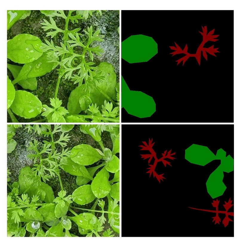
Qualitative Results

Here, we can visualize the qualitative results. The sequence of images is: Input Image, Ground Truth, and Prediction.

Observations:

Captures overall weed contours and structure quite well.
Handles complex textures and occlusions with reasonable accuracy.
No major confusion between background and weed classes.

Areas for Improvement:

Minor misses in small or isolated weed patches.
Slight class imbalance is visible — red class seems more confidently predicted than green.
Could benefit from:
- More training epochs
- Data augmentation focusing on a small region highlighting
- Post-processing (e.g., CRFs or morphological ops)

Conclusion

In this blog, we built a U-Net-based multi-class segmentation model from scratch using PyTorch. We trained it on an agricultural weed dataset and evaluated its performance using both qualitative and quantitative metrics. The model is lightweight, accurate, and efficient — making it suitable for real-world deployment in precision agriculture.

If you found this helpful, consider starring the GitHub repo or sharing it with others working in computer vision!”

Code: Multiclass Segmentation in PyTorch

Next Steps / Future Work

Add test-time augmentations for a further boost in accuracy
Try transfer learning by using a pre-trained encoder (e.g., ResNet)

What is Multiclass Segmentation?

Project Structure

Dataset

Class Color Mapping:

Model: U-Net Architecture

Imports

Convolutional Blocks

Encoder Block: Downsampling

Decoder Blocks: Upsampling + Skip Connection

U-Net Model

Utility Functions

Loss Functions

Dice Loss

Dice + CrossEntropy Loss

Why Use Dice + Cross Entropy?

Training Pipeline

Imports

Loading Dataset

Dataset Class

Training Function

Validation Function

Execution: Training the U-Net

Model Evaluation and Visualization

Imports

Convert Class Index to RGB

Evaluation Function

Main Execution

Quantitative Results

Qualitative Results

Conclusion

Next Steps / Future Work

Related Post

Leave a Reply Cancel reply