Object detection is a fundamental task in computer vision that involves identifying and locating objects within an image or video. In this post, we will be discussing a simple method for object detection using bounding box regression in TensorFlow.
Bounding box regression is a technique used to predict the location of an object in an image by training a model to predict the coordinates of the bounding box surrounding the object. This method is simple to implement and provides a good starting point. In this post, we will go over the basic of object detection and try to implement a simple object detection from scratch in TensorFlow using the pre-trained MobileNetv2.
What is Object Detection
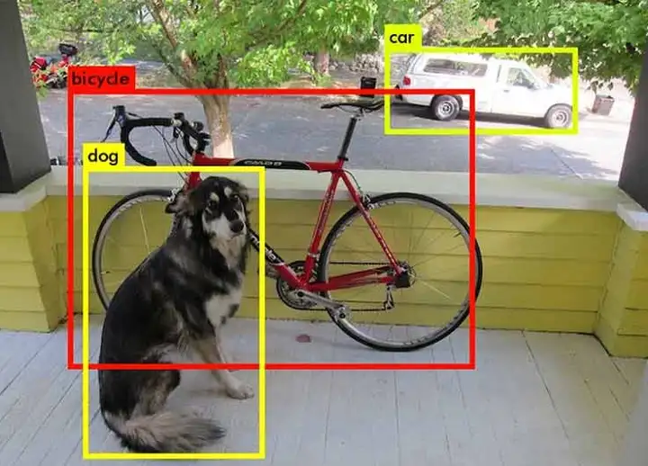
Object detection is a technique in computer vision that aims at identifying and locating objects within an image or video. In other words, it’s a way for computers to recognize and locate specific things, such as a person, a car, or a building, within a picture or a video.
Object detection is the task of identifying and locating objects within an image or video using a convolutional neural network (CNN) for feature extraction and predicting bounding boxes for object localization and class label for object classification.
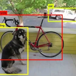
For example, imagine you have a picture of a street with cars, buildings, and people. An object detection algorithm would be able to identify each car, building, and person in the picture and draw a box around them, indicating where they are located in the image. This can be very useful for various applications such as self-driving cars, security cameras, and even social media tagging.
Dataset
For this tutorial, I had build a simple dataset on Human Detection. The dataset contains 847 images, where each image is having only one bounding box. The bounding box contains the four coordinates points – [x1, y1, x2, y2]. Here,
- [x1, y1] refers to the top-left point of the bounding box.
- [x2, y2] refers to the bottom-right point of the bounding box.
Download the dataset from here: Human Detection
The dataset contains the following files:
- images – This folder contains 847 images.
- bbox.csv – This CSV file stores the image name and its bounding box coordinate points, i.e., x1, y1, x2, y2.
For this tutorial, we split the complete dataset into training, validation and testing. Here
- Training dataset: 80% images and bounding boxes.
- Validation dataset: 10% images and bounding boxes.
- Testing dataset: 10% images and bounding boxes.
Dataset Preprocessing
The model would use the image as the input and predicts the four values (bounding box coordinate points). Before moving on to the training part, we need to understand the pre-processing of both the images and the bounding box.
We normalize the image by converting its pixels from 0 to 255 to the range of -1 and +1. This is a normalization technique which is used by MobileNetv2. You can change it according to your use.
We normalize the bounding box values by dividing them by the with and height of the image. This would convert the bounding box value in the range of 0 and 1.
- normalized x1 = x1 / image width
- normalized y1 = y1 / image height
- normalized x2 = x2 / image width
- normalized y2 = y2 / image height
Let’s understand this with an example.
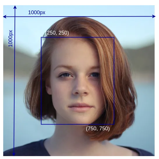
In the above image, we are given the height and width of the image along with its bounding box values.
- height – 1000 pixels
- width – 1000 pixels
Bounding box = [250, 250, 750, 750]
- x1 – 250
- y1 – 250
- x2 – 750
- y2 – 750
Let’s normalize them
normalized x1 = 250/1000 = 0.25
normalized y1 = 250/1000 = 0.25
normalized x2 = 750/1000 = 0.75
normalized y2 = 750/1000 = 0.75
Normalized bounding box = [0.25, 0.25, 0.75, 0.75]
Object Detection Architecture
We will use the pre-trained MobileNetv2 as the backbone to build our object detection architecture. After that, we will integrate a detection head to predict the bounding box.

from tensorflow.keras import layers as L
from tensorflow.keras.models import Model
from tensorflow.keras.applications import MobileNetV2

def build_model(input_shape):
    """ Inputs """
    inputs = L.Input(input_shape)

    """ Backbone """
    backbone = MobileNetV2(
        include_top=False,
        weights="imagenet",
        input_tensor=inputs,
        alpha=1.0
    )
    backbone.trainable = False
    # backbone.summary()

    """ Detection Head """
    x = backbone.output
    x = L.Conv2D(256, kernel_size=1, padding="same")(x)
    x = L.BatchNormalization()(x)
    x = L.Activation("relu")(x)
    x = L.GlobalAveragePooling2D()(x)
    x = L.Dropout(0.5)(x)
    x = L.Dense(4, activation="sigmoid")(x)

    """ Model """
    model = Model(inputs, x)
    return model
Training the Object Detection Model
We will begin by importing all the required libraries.
import os
os.environ["TF_CPP_MIN_LOG_LEVEL"] = "2"

import numpy as np
import cv2
from glob import glob
import tensorflow as tf
from tensorflow.keras.callbacks import ModelCheckpoint, CSVLogger, ReduceLROnPlateau, EarlyStopping, TensorBoard
from tensorflow.keras.optimizers import Adam
from sklearn.model_selection import train_test_split
from model import build_model
Now, we will define two global parameters – height and width as 512 x 512. These parameters can be accessed by any function directly.
""" Global parameters """
H = 512
W = 512
Next, we define our function called create_dir. This function helps us to create empty folders, which are used to save model checkpoints and log files.
def create_dir(path):
    if not os.path.exists(path):
        os.makedirs(path)
Now, we will build the load_dataset function which takes the dataset path and a split value as arguments. The function is used to load the dataset and split it into training, validation and testing.
def load_dataset(path, split=0.1):
    """ Extracting the images and bounding boxes from csv file. """
    images = []
    bboxes = []

    df = pd.read_csv(os.path.join(path, "bbox.csv"))
    for index, row in df.iterrows():
        name = row["name"]
        x1 = int(row["x1"])
        y1 = int(row["y1"])
        x2 = int(row["x2"])
        y2 = int(row["y2"])

        image = os.path.join(path, "images", name)
        bbox = [x1, y1, x2, y2]

        images.append(image)
        bboxes.append(bbox)

    """ Split into training, validation and testing. """
    split_size = int(len(images) * split)

    train_x, valid_x = train_test_split(images, test_size=split_size, random_state=42)
    train_y, valid_y = train_test_split(bboxes, test_size=split_size, random_state=42)

    train_x, test_x = train_test_split(train_x, test_size=split_size, random_state=42)
    train_y, test_y = train_test_split(train_y, test_size=split_size, random_state=42)

    return (train_x, train_y), (valid_x, valid_y), (test_x, test_y)
The load function first loads all the image path and bounding box values from the CSV file. After that, it split them into proper training, validation and testing datasets.
Next, we have a function called read_image_bbox. The function does the following tasks:
- Read the image and resize it.
- Normalize the image to the range of -1 and +1.
- Normalize the bounding box values by dividing them by the original image height and width.
def read_image_bbox(path, bbox):
    """ Image """
    path = path.decode()
    image = cv2.imread(path, cv2.IMREAD_COLOR)
    h, w, _ = image.shape
    image = cv2.resize(image, (W, H))
    image = (image - 127.5) / 127.5 ## [-1, +1]
    image = image.astype(np.float32)

    """ Bounding box """
    x1, y1, x2, y2 = bbox

    norm_x1 = float(x1/w)
    norm_y1 = float(y1/h)
    norm_x2 = float(x2/w)
    norm_y2 = float(y2/h)
    norm_bbox = np.array([norm_x1, norm_y1, norm_x2, norm_y2], dtype=np.float32)

    return image, norm_bbox
Now, we will use the above read_image_bbox function along with some other functions to build the dataset pipeline using tf.data API.
Now, we are going to implement the parse and tf_dataset functions. The parse function would use the read_image_bbox function and allows us to use it in the TensorFlow environment. As the read_image_bbox contains the code written using OpenCV and NumPy, which are libraries outside the TensorFlow.
def parse(x, y):
    x, y = tf.numpy_function(read_image_bbox, [x, y], [tf.float32, tf.float32])
    x.set_shape([H, W, 3])
    y.set_shape([4])
    return x, y

def tf_dataset(images, bboxes, batch=8):
    ds = tf.data.Dataset.from_tensor_slices((images, bboxes))
    ds = ds.map(parse).batch(batch).prefetch(10)
    return ds
Now, we will start with the execution of the functions to begin the training process. First of all, we begin by seeding the environment. This is done to ensure that the random numbers generated during the training process are consistent and reproducible. Thus making the training process more predictable and reproducible.
if __name__ == "__main__":
    """ Seeding """
    np.random.seed(42)
    tf.random.set_seed(42)

    """ Directory for storing files """
    create_dir("files")

    """ Hyperparameters """
    batch_size = 16
    lr = 1e-4
    num_epochs = 500
    model_path = os.path.join("files", "model.h5")
    csv_path = os.path.join("files", "log.csv")
Along with seeding, we have also created an empty folder called files. This folder would store the model checkpoint and the log file. After that, we defined the hyperparameters.
Next, we will load the dataset and use the tf_dataset function to create the training and validation dataset pipeline.
""" Dataset """
    dataset_path = "../Human-Detection"
    (train_x, train_y), (valid_x, valid_y), (test_x, test_y) = load_dataset(dataset_path)
    print(f"Train: {len(train_x)} - {len(train_y)}")
    print(f"Valid: {len(valid_x)} - {len(valid_y)}")
    print(f"Test : {len(test_x)} - {len(test_y)}")

    train_ds = tf_dataset(train_x, train_y, batch=batch_size)
    valid_ds = tf_dataset(valid_x, valid_y, batch=batch_size)
Now, we are going to build and compile our object detection model.
    """ Model """
    model = build_model((H, W, 3))
    model.compile(
        loss="binary_crossentropy",
        optimizer=Adam(lr)
    )
As the model is using the sigmoid as the output activation, so we will use binary_crossentropy as the loss function. You can also try mse (mean squared error) as the loss function.
Next, we defined some callback and call the model.fit to start the training.
    callbacks = [
        ModelCheckpoint(model_path, verbose=1, save_best_only=True),
        ReduceLROnPlateau(monitor='val_loss', factor=0.1, patience=5, min_lr=1e-7, verbose=1),
        CSVLogger(csv_path, append=True),
        EarlyStopping(monitor='val_loss', patience=20, restore_best_weights=False),
    ]

    model.fit(
        train_ds,
        epochs=num_epochs,
        validation_data=valid_ds,
        callbacks=callbacks
    )
You can download the model checkpoint from here: mode.h5
Before moving on to the testing part. Let us first understand the Intersection over Union.
Intersection over Union
Intersection over Union (IoU) is a common evaluation metric used in object detection to measure the accuracy of the predicted bounding boxes. It compares the predicted bounding box with the ground truth bounding box and calculates the ratio of the area of the intersection to the area of the union.
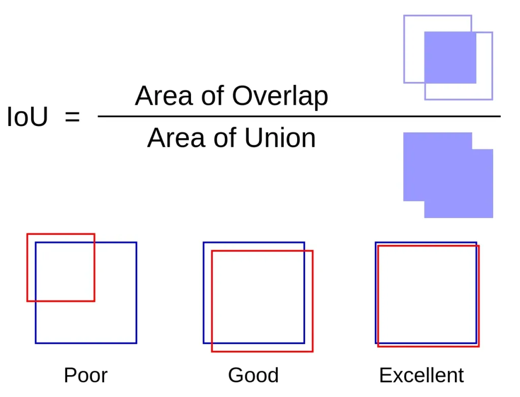
In other words, it measures the overlap between the predicted bounding box and the ground truth bounding box. A higher IoU value indicates that the predicted bounding box is a better match for the ground truth bounding box, thus providing a more accurate object detection. The IoU values range from 0 to 1, with a perfect match having an IoU value of 1 and no match having an IoU value of 0.
Testing – Prediction and Evaluation
As the training is over, so we will test our object detection model on the test dataset and calculate the mean IoU (Intersection over Union).
Let us first import all the required libraries.
import os
os.environ["TF_CPP_MIN_LOG_LEVEL"] = "2"

import numpy as np
import cv2
from tqdm import tqdm
import tensorflow as tf
from train import load_dataset, create_dir
Again we will define the height and width at the top, so that other functions can use it directly.
""" Global parameters """
H = 512
W = 512
Now, we will define the cal_iou function. This function helps us to calculate the Intersection over Union (IoU) between the true and predicted bounding box.
def cal_iou(y_true, y_pred):
    x1 = max(y_true[0], y_pred[0])
    y1 = max(y_true[1], y_pred[1])
    x2 = min(y_true[2], y_pred[2])
    y2 = min(y_true[3], y_pred[3])

    intersection_area = max(0, x2 - x1 + 1) * max(0, y2 - y1 + 1)

    true_area = (y_true[2] - y_true[0] + 1) * (y_true[3] - y_true[1] + 1)
    bbox_area = (y_pred[2] - y_pred[0] + 1) * (y_pred[3] - y_pred[1] + 1)

    iou = intersection_area / float(true_area + bbox_area - intersection_area)
    return iou
Now, we will begin with the execution of the functions. We will first seed the environment and create an empty folder called results. This folder would store the test images with both true and predicted bounding boxes along with the IoU score.
if __name__ == "__main__":
    """ Seeding """
    np.random.seed(42)
    tf.random.set_seed(42)

    """ Directory for storing files """
    create_dir("results")
Next, we will load our model using the checkpoint file named model.h5
    """ Load the model """
    model = tf.keras.models.load_model(os.path.join("files", "model.h5"))
Next, we will load the dataset and use the test set for prediction and evaluation.
    """ Dataset """
    dataset_path = "../Human-Detection"
    (train_x, train_y), (valid_x, valid_y), (test_x, test_y) = load_dataset(dataset_path)
    print(f"Train: {len(train_x)} - {len(train_y)}")
    print(f"Valid: {len(valid_x)} - {len(valid_y)}")
    print(f"Test : {len(test_x)} - {len(test_y)}")
Now, we will begin with the process of prediction and evaluation.
First, we will define an empty list called mean_iou and the loop over the test images and test masks.
    mean_iou = []
    for image, true_bbox in tqdm(zip(test_x, test_y), total=len(test_y)):
Inside the loop, we will first extract the name from the image path and then read the image and normalize it.
        """ Extracting the name """
        name = image.split("/")[-1]

        """ Reading the image """
        image = cv2.imread(image, cv2.IMREAD_COLOR)
        x = cv2.resize(image, (W, H))
        x = (x - 127.5) / 127.5
        x = np.expand_dims(x, axis=0)
Next, we will extract the true bounding box values from the true_bbox.
        """ True bounding box """
        true_x1, true_y1, true_x2, true_y2 = true_bbox
After that, we use the normalized image to predict the bounding box. We then rescale the normalized bounding box coordinate points into a proper un-normalized value which can be used to plot the bounding box on the image.
        """ Rescale the bbox points. """
        pred_x1 = int(pred_bbox[0] * image.shape[1])
        pred_y1 = int(pred_bbox[1] * image.shape[0])
        pred_x2 = int(pred_bbox[2] * image.shape[1])
        pred_y2 = int(pred_bbox[3] * image.shape[0])
Next, we calculate the IoU and append it to the mean_iou list.
        """ Calculate IoU """
        iou = cal_iou(true_bbox, [pred_x1, pred_y1, pred_x2, pred_y2])
        mean_iou.append(iou)
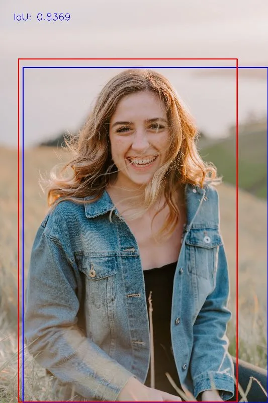
Now, we have both the true and predicted bounding box. We will plot them on the original input image. The true bounding box is in blue and the predicted one is in red.
        """ Plot them on image """
        image = cv2.rectangle(image, (true_x1, true_y1), (true_x2, true_y2), (255, 0, 0), 10) ## BLUE
        image = cv2.rectangle(image, (pred_x1, pred_y1), (pred_x2, pred_y2), (0, 0, 255), 10) ## RED
Next, we will also write the IoU score on the image and finally save the image to the results folder.
        x = int(image.shape[1] * 0.05)
        y = int(image.shape[0] * 0.05)
        font_size = int(image.shape[0] * 0.001)
        cv2.putText(image, f"IoU: {iou:.4f}", (x, y), cv2.FONT_HERSHEY_SIMPLEX, font_size, (255, 0, 0), 3)

        """ Saving the image """
        cv2.imwrite(f"results/{name}", image)
Finally, in the end, we calculate the mean IOU of all the images and print it on the screen.
    """ Mean IoU """
    score = np.mean(mean_iou, axis=0)
    print(f"Mean IoU: {score:.4f}")
Results

Summary
In this tutorial, we have implemented a very basic object detector using the pre-trained Mobilenetv2. We have trained the model on the bounding box regression technique to predict the bounding box.
I hope you learn the basic of object detection from this tutorial. You can follow us on:

Hi Nikhil,
Thanks for your dedications and explored very well. it is great helps to me.
by
Palani