Today, in this blog post, we will learn how to train a Convolutional Neural Network (CNN) to detect human facial landmarks, such as eyes, mouth, nose, jawline and more. We will use the pre-trained MobileNetv2 from TensorFlow to build our model and then train it on Landmark Guided Face Parsing (LaPa) dataset.
Outline
- What are Facial Landmarks?
- Landmark Guided Face Parsing Dataset
- Implementation
- Summary
What are Facial Landmarks?
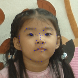
Facial landmarks are the key points which represent the different facial structures, such as eyes, nose, lips, mouth, jawline and more. The combination of all the key points together constitutes the facial landmarks and these landmarks can be used in different computer vision tasks such as identifying gaze direction, detecting facial gestures, and swapping faces.
These landmarks are simple coordinates points (x and y) which depict a specific region of the human face. The number of facial landmarks points can differ depending on the dataset and the complexity of the task to be performed.
Facial landmark detection is a computer vision task in which we input the human face and the model is going to predict landmarks.
In this tutorial, we will train a pre-trained MobileNetv2 to predict 106 landmarks for a human face.
Landmark Guided Face Parsing Dataset
The dataset contains more than 22,000 facial images with abundant variations in expression, pose and occlusion and each image of the dataset is provided with an 11-category pixel-level label map and 106-point landmarks.

To learn more about the dataset please read the research paper: A New Dataset and Boundary-Attention Semantic Segmentation for Face Parsing
Implementation
Now, we will start with the implementation, where we will first begin by training the model on the Landmark Guided Face Parsing (LaPa) dataset and then testing it.
Training – train.py
The training file contains the code for loading the dataset and then building the dataset pipeline using the tf.data API. Next, we use the pre-trained MobileNetv2 to build the model and at last, we train the model.
We import all the required libraries and functions.
import os
os.environ["TF_CPP_MIN_LOG_LEVEL"] = "2"

import numpy as np
import cv2
from glob import glob

import tensorflow as tf
from tensorflow.keras import layers as L
from tensorflow.keras.applications import MobileNetV2
from tensorflow.keras.callbacks import ModelCheckpoint, ReduceLROnPlateau, EarlyStopping, CSVLogger
Next, we define some global variables.
global image_h
global image_w
global num_landmarks
During training, we need to save the model.h5 weight file. So, we will define a function called create_dir to create a folder or directory.
def create_dir(path):
    if not os.path.exists(path):
        os.makedirs(path)
We will now define the load_dataset function, which is going to load training, validation and testing datasets. Each of the dataset folders contains the following sub-folders:
- images – contains the images as .jpg files.
- labels – contains the segmentation mask.
- landmarks – contains the text file, which has the landmarks (coordinate points).
def load_dataset(path):
    train_x = sorted(glob(os.path.join(path, "train", "images", "*.jpg")))
    train_y = sorted(glob(os.path.join(path, "train", "landmarks", "*.txt")))

    valid_x = sorted(glob(os.path.join(path, "val", "images", "*.jpg")))
    valid_y = sorted(glob(os.path.join(path, "val", "landmarks", "*.txt")))

    test_x = sorted(glob(os.path.join(path, "test", "images", "*.jpg")))
    test_y = sorted(glob(os.path.join(path, "test", "landmarks", "*.txt")))

    return (train_x, train_y), (valid_x, valid_y), (test_x, test_y)
Now, we have loaded the dataset, so we will define a function to read the image and the landmark text file.
def read_image_lankmarks(image_path, landmark_path):
    """ Image """
    image = cv2.imread(image_path, cv2.IMREAD_COLOR)
    h, w, _ = image.shape
    image = cv2.resize(image, (image_w, image_h))
    image = image/255.0
    image = image.astype(np.float32)

    """ Lankmarks """
    data = open(landmark_path, "r").read()
    lankmarks = []

    for line in data.strip().split("\n")[1:]:
        x, y = line.split(" ")
        x = float(x)/w
        y = float(y)/h

        lankmarks.append(x)
        lankmarks.append(y)

    lankmarks = np.array(lankmarks, dtype=np.float32)

    return image, lankmarks
Now, we will create preprocess and tf_dataset functions that would help in building the dataset pipeline using the tf.data API.
def preprocess(x, y):
    def f(x, y):
        x = x.decode()
        y = y.decode()

        image, landmarks = read_image_lankmarks(x, y)
        return image, landmarks

    image, landmarks = tf.numpy_function(f, [x, y], [tf.float32, tf.float32])
    image.set_shape([image_h, image_w, 3])
    landmarks.set_shape([num_landmarks * 2])

    return image, landmarks

def tf_dataset(x, y, batch=8):
    ds = tf.data.Dataset.from_tensor_slices((x, y))
    ds = ds.shuffle(buffer_size=5000).map(preprocess)
    ds = ds.batch(batch).prefetch(2)
    return ds
Now, we will build our model using the pre-trained MobileNetv2.
def build_model(input_shape, num_landmarks):
    inputs = L.Input(input_shape)

    backbone = MobileNetV2(include_top=False, weights="imagenet", input_tensor=inputs, alpha=0.5)
    backbone.trainable = True

    x = backbone.output
    x = L.GlobalAveragePooling2D()(x)
    x = L.Dropout(0.2)(x)
    outputs = L.Dense(num_landmarks*2, activation="sigmoid")(x)

    model = tf.keras.models.Model(inputs, outputs)
    return model
Till now, we have defined all the functions required for training the model. Now, we will begin with the execution of the functions
First, we will seed the environment, create a folder and define some hyperparameters.
if __name__ == "__main__":
    """ Seeding """
    np.random.seed(42)
    tf.random.set_seed(42)

    """ Directory for storing files """
    create_dir("files")

    """ Hyperparameters """
    image_h = 512
    image_w = 512
    num_landmarks = 106
    input_shape = (image_h, image_w, 3)
    batch_size = 32
    lr = 1e-3
    num_epochs = 100

    """ Paths """
    dataset_path = "dataset/LaPa"
    model_path = os.path.join("files", "model.h5")
    csv_path = os.path.join("files", "data.csv")
Next, we will load the dataset by giving the dataset_path and then build the training and validation dataset using the tf_datset function.
    """ Loading the dataset """
    (train_x, train_y), (valid_x, valid_y), (test_x, test_y) = load_dataset(dataset_path)
    print(f"Train: {len(train_x)}/{len(train_y)} - Valid: {len(valid_x)}/{len(valid_y)} - Test: {len(test_x)}/{len(test_x)}")
    print("")

    """ Dataset Pipeline """
    train_ds = tf_dataset(train_x, train_y, batch=batch_size)
    valid_ds = tf_dataset(valid_x, valid_y, batch=batch_size)
Now, we call our build_model function and compile it by providing the loss function and the optimizer.
    """ Model """
    model = build_model(input_shape, num_landmarks)
    model.compile(loss="binary_crossentropy", optimizer=tf.keras.optimizers.Adam(lr))
At last, we will define the callbacks and call the model.fit to begin the training.
    """ Training """
    callbacks = [
        ModelCheckpoint(model_path, verbose=1, save_best_only=True, monitor='val_loss'),
        ReduceLROnPlateau(monitor='val_loss', factor=0.1, patience=5, min_lr=1e-7, verbose=1),
        CSVLogger(csv_path, append=True),
        EarlyStopping(monitor='val_loss', patience=20, restore_best_weights=False)
    ]

    model.fit(train_ds,
        validation_data=valid_ds,
        epochs=num_epochs,
        callbacks=callbacks
    )
Testing – test.py
Now the model is trained and we have the model.h5 weight file saved in the files folder along with the data.csv file.
So, first of all, we will import all the required libraries and functions. After that, we will define some global variables.
import os
os.environ["TF_CPP_MIN_LOG_LEVEL"] = "2"

import numpy as np
import cv2
from glob import glob
from tqdm import tqdm
import tensorflow as tf
from train import create_dir, load_dataset

global image_h
global image_w
global num_landmarks
Next, we will define a function called plot_landmarks, which would take the following arguments:
- image – the image on which the landmarks are to be plotted.
- landmarks – these are the normalized x and y coordinates in the form of a list.
def plot_lankmarks(image, landmarks):
    h, w, _ = image.shape
    radius = int(h * 0.005)

    for i in range(0, len(landmarks), 2):
        x = int(landmarks[i] * w)
        y = int(landmarks[i+1] * h)

        image = cv2.circle(image, (x, y), radius, (255, 0, 0), -1)

    return image
The landmarks list contains the coordinates in the following formats: [x1, y1, x2, y2, x3, y3,..] and so on. Due to this, we loop over the landmarks list with an increment of two to get the x and y points.
All these coordinates are normalized, meaning that their values lie between 0 and 1. So, we multiply them by the width and height and convert them to integers. We use these integer coordinate points and plot them on the input image.
Next, we will begin with the execution of the test.py.
if __name__ == "__main__":
    """ Seeding """
    np.random.seed(42)
    tf.random.set_seed(42)

    """ Directory for storing files """
    create_dir("results")

    """ Hyperparameters """
    image_h = 512
    image_w = 512
    num_landmarks = 106

    """ Paths """
    dataset_path = "/media/nikhil/Seagate Backup Plus Drive/ML_DATASET/LaPa"
    model_path = os.path.join("files", "model.h5")

    """ Loading the dataset """
    (train_x, train_y), (valid_x, valid_y), (test_x, test_y) = load_dataset(dataset_path)
    print(f"Train: {len(train_x)}/{len(train_y)} - Valid: {len(valid_x)}/{len(valid_y)} - Test: {len(test_x)}/{len(test_x)}")
    print("")

    """ Load the model """
    model = tf.keras.models.load_model(model_path)
    # model.summary()
Now, we have loaded our trained model. We will use it to predict the landmarks on the test images.
    """ Prediction """
    for x, y in tqdm(zip(test_x, test_y), total=len(test_x)):
        """ Extract the name """
        name = x.split("/")[-1].split(".")[0]

        """ Reading the image """
        image = cv2.imread(x, cv2.IMREAD_COLOR)
        image_x = image
        image = cv2.resize(image, (image_w, image_h))
        image = image/255.0 ## (512, 512, 3)
        image = np.expand_dims(image, axis=0) ## (1, 512, 512, 3)
        image = image.astype(np.float32)

        """ Landmarks """
        data = open(y, "r").read()
        landmarks = []
        for line in data.strip().split("\n")[1:]:
            x, y = line.split(" ")
            x = float(x)/image_x.shape[1]
            y = float(y)/image_x.shape[0]

            landmarks.append(x)
            landmarks.append(y)

        landmarks = np.array(landmarks, dtype=np.float32)

        """ Prediction """
        pred = model.predict(image, verbose=0)[0]
        pred = pred.astype(np.float32)

        """ Saving the results """
        gt_landmarks = plot_lankmarks(image_x.copy(), landmarks)
        pred_landmarks = plot_lankmarks(image_x.copy(), pred)
        line = np.ones((image_x.shape[0], 10, 3)) * 255

        cat_images = np.concatenate([gt_landmarks, line, pred_landmarks], axis=1)
        cv2.imwrite(f"results/{name}.png", cat_images)
In the above code, we read the image, resize and normalize it. Then we read the landmarks from the text file and normalize them by dividing the x and y points by the width and height of the image.
The normalized image is fed to the model which predicts the normalized landmarks. We plot both the real and predicted landmarks on the image.
Results
A few examples show the comparison and the real and the predicted landmarks.

Summary
In this blog post, we have built a human face landmark detector using the pre-trained MobileNetv2. The model takes the human face and predicts the 106 landmarks. To learn about it in detail, please watch the YouTube tutorial: Human Face Landmark Detection in TensorFlow using MobileNetv2
Hopefully, I was able to give you some new information and you learn something from this article.
If YES, then, Follow me:


One thought on “Human Face Landmark Detection in TensorFlow using Pre-trained MobileNetv2”