ColonSegNet Implementation In TensorFlow

In this article, we will explore the technical intricacies of implementing ColonSegNet in TensorFlow. ColonSegNet is a lightweight, real-time colon segmentation architecture that has garnered attention for its efficiency in medical image analysis. In our previous post, we introduced the architecture and its components. Now, let’s explore the technical intricacies of implementing ColonSegNet in TensorFlow.

Previous Post: ColonSegNet: A Lightweight Real-Time Colon Segmentation Architecture

Install TensorFlow

pip install tensorflow

Now, let’s go through the code step by step.

Importing Libraries and Functions

Import necessary libraries and suppress TensorFlow warnings.

import os
os.environ["TF_CPP_MIN_LOG_LEVEL"] = "2"
from tensorflow.keras.layers import Conv2D, BatchNormalization, Activation, UpSampling2D, Dense
from tensorflow.keras.layers import GlobalAveragePooling2D, Conv2DTranspose, Concatenate, Input
from tensorflow.keras.layers import MaxPool2D
from tensorflow.keras.models import Model

The code starts by importing essential libraries. The os.environ line is used to suppress unnecessary TensorFlow warnings for cleaner output.

Squeeze and Excitation (SE) Block

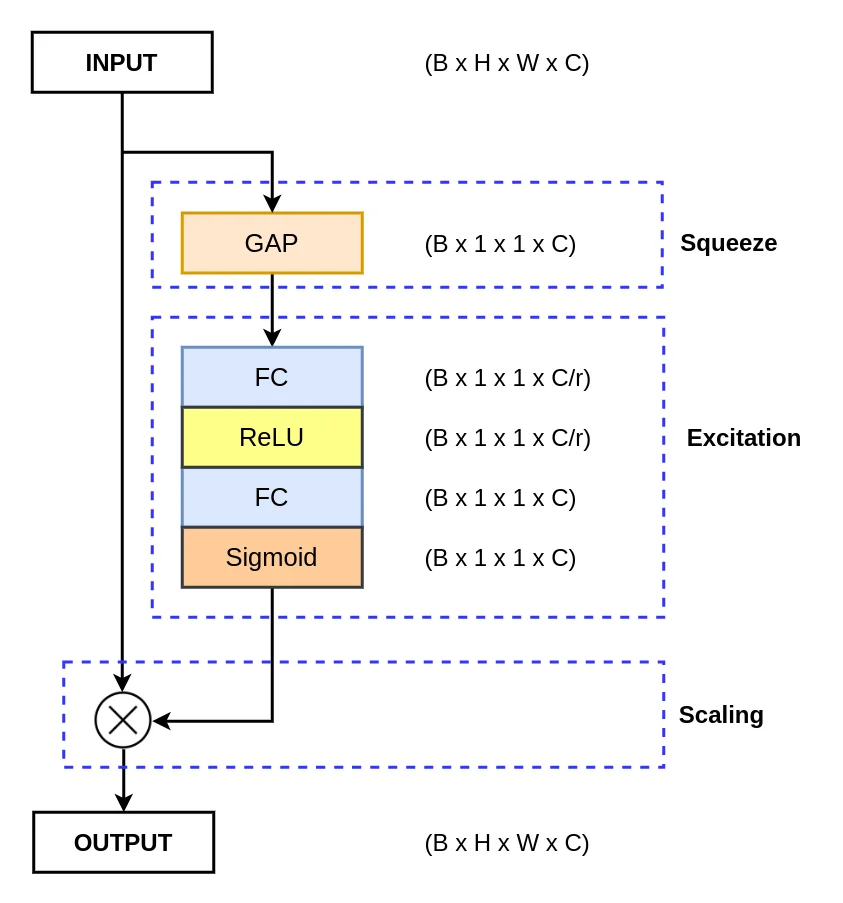
The se_layer function defines the Squeeze and Excitation Block block, a key component in enhancing the representational power of ColonSegNet. Let’s break down its implementation:

def se_layer(x, num_filters, reduction=16):
    x_init = x

    x = GlobalAveragePooling2D()(x)
    x = Dense(num_filters//reduction, use_bias=False, activation="relu")(x)
    x = Dense(num_filters, use_bias=False, activation="sigmoid")(x)
    x = x * x_init
    return x

• Global Average Pooling: It reduces the input tensor’s spatial dimensions to a single value per channel, capturing the global context.
• Squeeze: A fully connected layer with a ReLU activation compresses the channel-wise information, preparing it for excitation.
• Excitation: Another fully connected layer with a sigmoid activation produces a channel-wise scaling factor, indicating the importance of each channel.
• Scaling: The excitation output scales the input tensor element-wise, allowing the network to focus on relevant channels.

Read More:

• Squeeze and Excitation Networks
• What is Residual Network or ResNet?

Residual Block

The residual_block function represents a residual block, a crucial element in overcoming the vanishing gradient problem and facilitating information flow. Let’s explore its details:

def residual_block(x, num_filters):
    x_init = x

    x = Conv2D(num_filters, 3, padding="same")(x)
    x = BatchNormalization()(x)
    x = Activation("relu")(x)
    
    x = Conv2D(num_filters, 3, padding="same")(x)
    x = BatchNormalization()(x)

    s = Conv2D(num_filters, 1, padding="same")(x_init)
    s = BatchNormalization()(s)
    s = se_layer(s, num_filters)

    x = Activation("relu")(x + s)
    return x

• The block starts with a convolutional layer, followed by batch normalization and ReLU activation.
• Another convolutional layer is applied, and batch normalization is performed again.
• A shortcut connection is created using a 1×1 convolution followed by batch normalization and the SE layer.
• The final output is obtained by adding the shortcut connection to the output of the second convolutional layer, followed by ReLU activation.

Strided Convolution Block

The strided_conv_block function defines a block with strided convolution, aiding in downsampling spatial dimensions. This is crucial for capturing hierarchical features.

def strided_conv_block(x, num_filters):
    x = Conv2D(num_filters, 3, strides=2, padding="same")(x)
    x = BatchNormalization()(x)
    x = Activation("relu")(x)
    return x

Encoder Block

The encoder_block function combines the residual and strided convolution blocks to create an encoder block. It captures and refines features while downsampling the input.

def encoder_block(x, num_filters):
    x1 = residual_block(x, num_filters)
    x2 = strided_conv_block(x1, num_filters)
    x3 = residual_block(x2, num_filters)
    p = MaxPool2D((2, 2))(x3)

    return x1, x3, p

ColonSegNet Architecture

The build_colonsegnet function assembles the complete ColonSegNet architecture. It consists of encoder and decoder blocks, making it capable of segmenting colon regions in medical images.

def build_colonsegnet(input_shape):
    """ Input """
    inputs = Input(input_shape)

    """ Encoder """
    s11, s12, p1 = encoder_block(inputs, 64)
    s21, s22, p2 = encoder_block(p1, 256)

    """ Decoder 1 """
    x = Conv2DTranspose(128, 4, strides=4, padding="same")(s22)
    x = Concatenate()([x, s12])
    x = residual_block(x, 128)
    r1 = x

    x = Conv2DTranspose(128, 4, strides=2, padding="same")(s21)
    x = Concatenate()([x, r1])
    x = residual_block(x, 128)

    """ Decoder 2 """
    x = Conv2DTranspose(64, 4, strides=2, padding="same")(x)
    x = Concatenate()([x, s11])
    x = residual_block(x, 64)
    r2 = x

    x = Conv2DTranspose(32, 4, strides=2, padding="same")(s12)
    x = Concatenate()([x, r2])
    x = residual_block(x, 32)

    """ Output """
    output = Conv2D(1, 1, padding="same")(x)

    """ Model """
    model = Model(inputs, output)

    return model

Running the ColonSegNet

In the main block, we specify the input shape, build the ColonSegNet model using the defined function, and print the model summary.

if __name__ == "__main__":
    input_shape = (512, 512, 3)
    model = build_colonsegnet(input_shape)
    model.summary()

Conclusion

Congratulations! You’ve just explored the details of the implementation of ColonSegNet in TensorFlow. Feel free to experiment with the code, integrate it into your projects, and contribute to the growing field of medical image segmentation.

Happy coding!