In this article, you will learn to perform person segmentation with DeepLabV3+ architecture on human images. Here, we will cover the entire process of image segmentation starting from data processing to evaluation. The entire code is written in Python programming language using TensorFlow 2.5 framework.
Table of Content
- What is image segmentation?
- Person segmentation dataset.
- Data Processing.
- Loading the dataset.
- Split the dataset into training and testing.
- Data augmentation
- DeepLabV3+ architecture.
- Training the DeepLabV3+ architecture
- Evaluation on the model.
- Prediction on images from internet.
- Collecting images from internet.
- Predicting mask.
What is image segmentation?
Image segmentation is simply a process of dividing an image into different regions. Each region helps to identify different objects present in an image. Image segmentation is used to understand and interpret the image more efficiently. It is used in multiple applications. These applications include satellite imaging, medical imaging, self-driving cars and many more.
In the context of deep learning, image segmentation refers to the process of predicting a label for each pixel in the image. It helps in better localization of the object present in the image.
In this article, you would learn about binary image segmentation, where each image pixel can be classified into two classes either 0 or 1.
- 0 – refers to the background.
- 1 – refers to the foreground (main object).
Here, in this article, we would classify each image pixel into a background class or a human class.
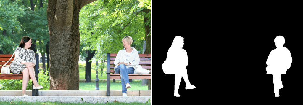
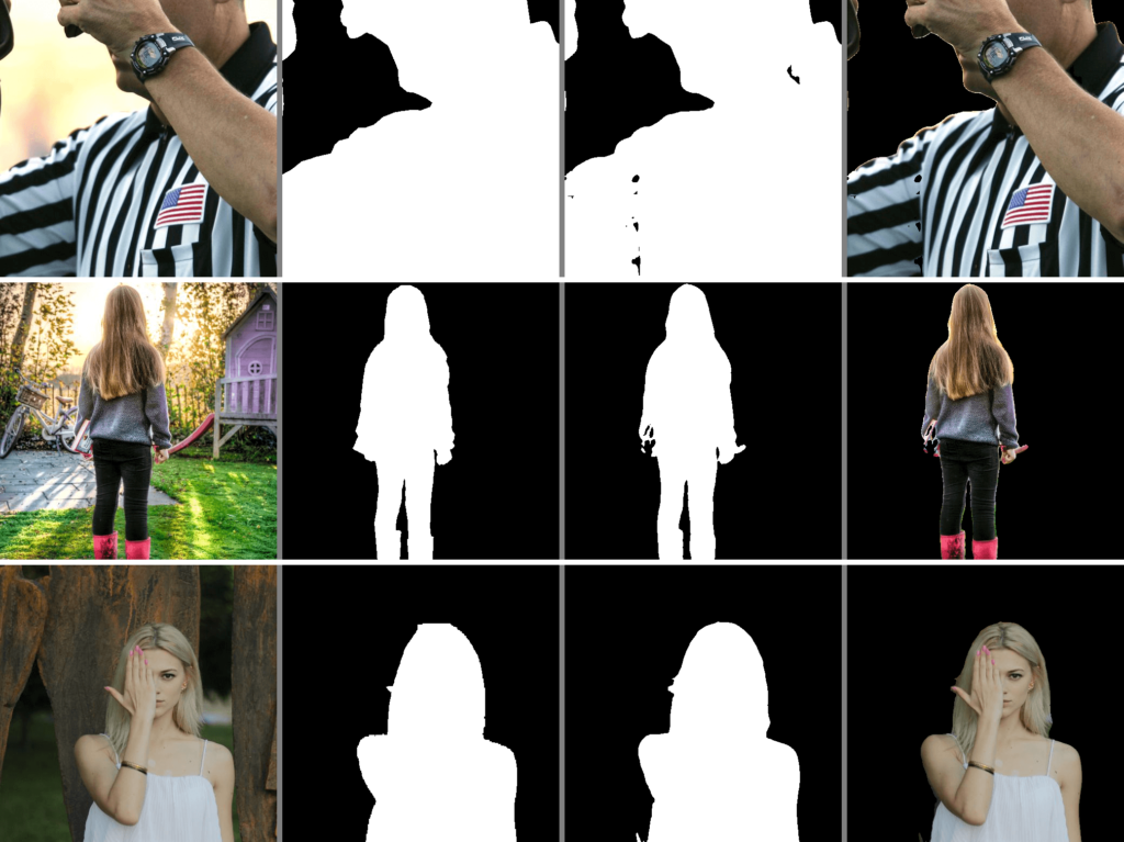
In the above figure, the left image is the RGB image and the right image is its respective ground truth mask. In the ground truth, the white region indicates the person.
We already have covered a few articles related to segmentation:
- Unet Segmentation in TensorFlow
- Polyp Segmentation using UNET in TensorFlow 2.0
- UNET Segmentation with Pretrained MobileNetV2 as Encoder
Person Segmentation Dataset
For the human image segmentation task, we need a dataset with human images and with properly annotated masks. Here we are going to use the Person Segmentation dataset from https://www.kaggle.com/nikhilroxtomar/person-segmentation. The dataset consists of 5,678 images and masks pairs.
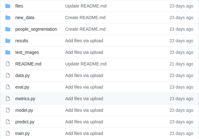
The dataset contains three folders:
- images – contain images.
- masks – contain masks.
- segmentation – contains three txt file.
- train.txt – contain training images names.
- trainval.txt – contain training and validation images names.
- val.txt – contain validation image names.
For this tutorial, we are not going to use these splits. We are going to use our own splits, where we will divide the complete dataset into training and validation/testing.
Data Processing
The data processing part deals with the following:
- Loading the dataset.
- Split the dataset into training and testing.
- Apply data augmentation.
All the code for the data processing would be in the data.py file. At the first, you need to import all the required libraries, classes and their functions.
data.py
import os
import numpy as np
import cv2
from glob import glob
from tqdm import tqdm
from sklearn.model_selection import train_test_split
from albumentations import HorizontalFlip, GridDistortion, OpticalDistortion, ChannelShuffle, CoarseDropout, CenterCrop, Crop, Rotate
As we are going to split the data and apply data augmentation. We also need to save the data into some folders. For this reason, we would write a function to create a required folder.
The function is called create_dir. This function takes a single parameter:
- path – the folders that needs to be created.
def create_dir(path):
    if not os.path.exists(path):
        os.makedirs(path)
The function creates the required folders if they do not exist.
Now we will create a function called load_data. This function do the following functions:
- Load all the images and masks paths.
- Split the data into training and testing.
The functions take two parameters:
- path – It is the path to the person segmentation dataset.
- split – It is the amount of data to be used for testing.
def load_data(path, split=0.1):Loading the dataset.
Here, we have loaded all the images and masks paths in the variables X and Y respectively.
    X = sorted(glob(os.path.join(path, "images", "*.jpg")))
    Y = sorted(glob(os.path.join(path, "masks", "*.png")))
Split the dataset into training and testing.
Here, we first calculate the test size and save it in a variable called split_size.
Next, we split the images and masks path present in the X and Y variable into training and testing data. Finally, we return the training and testing images and masks.
    split_size = int(len(X) * split)

    train_x, test_x = train_test_split(X, test_size=split_size, random_state=42)
    train_y, test_y = train_test_split(Y, test_size=split_size, random_state=42)

    return (train_x, train_y), (test_x, test_y)
Till now we have loaded the dataset and split it into the training and testing set. We can use this dataset for human image segmentation. As the training dataset is enough to get good results.
As we all know deep learning algorithms heavily depends upon the size of the training dataset. So, next, we are going to apply data augmentation techniques to the training dataset.
Data augmentation
In this part, we are going to create a function called augment_data. The function is going to perform the following functions:
- Resize the image and masks into a provided shape.
- Apply augmentation, if you want.
The function augment_data takes the following parameters:
- images – List of all the images path.
- masks – List of all the masks path.
- save_path – It is the path where data would be saved.
- augment – It is a boolean variable, if True data augmentation would be applied and False, then not.
def augment_data(images, masks, save_path, augment=True):
    H = 512
    W = 512
Now, we are going to loop over the images and masks path. Inside the loop we are going to do the following:
- Extracting the name from image path. As later we need to save the images.
- Reading the images and masks.
- Data augmentation.
- Resizing and saving the images and masks.
    for x, y in tqdm(zip(images, masks), total=len(images)):
        name = x.split("/")[-1].split(".")[0]

        x = cv2.imread(x, cv2.IMREAD_COLOR)
        y = cv2.imread(y, cv2.IMREAD_COLOR)
Now we are going to different augmentation techniques if the augment is set to True.
        if augment == True:
            aug = HorizontalFlip(p=1.0)
            augmented = aug(image=x, mask=y)
            x1 = augmented["image"]
            y1 = augmented["mask"]

            x2 = cv2.cvtColor(x, cv2.COLOR_RGB2GRAY)
            y2 = y

            aug = ChannelShuffle(p=1)
            augmented = aug(image=x, mask=y)
            x3 = augmented['image']
            y3 = augmented['mask']

            aug = CoarseDropout(p=1, min_holes=3, max_holes=10, max_height=32, max_width=32)
            augmented = aug(image=x, mask=y)
            x4 = augmented['image']
            y4 = augmented['mask']

            aug = Rotate(limit=45, p=1.0)
            augmented = aug(image=x, mask=y)
            x5 = augmented["image"]
            y5 = augmented["mask"]

            X = [x, x1, x2, x3, x4, x5]
            Y = [y, y1, y2, y3, y4, y5]

        else:
            X = [x]
            Y = [y]
The augmentation is applied and we have all the images and masks array in the X and Y variables. We would now begin resizing and then saving the data.
Now, we apply a for loop over the X and Y variables. Next, on each individual image and mask array i and m, we will first try to apply a center cropping on them. Center cropping helps to prevent unnecessary stretching and squeezing. If any error occurred while applying center cropping, then we would directly, resize the image and mask using the OpenCV cv2.resize() function.
Then we save the images and masks into a proper directory.
        index = 0
        for i, m in zip(X, Y):
            try:
                """ Center Cropping """
                aug = CenterCrop(H, W, p=1.0)
                augmented = aug(image=i, mask=m)
                i = augmented["image"]
                m = augmented["mask"]

            except Exception as e:
                i = cv2.resize(i, (W, H))
                m = cv2.resize(m, (W, H))

            tmp_image_name = f"{name}_{index}.png"
            tmp_mask_name = f"{name}_{index}.png"

            image_path = os.path.join(save_path, "image", tmp_image_name)
            mask_path = os.path.join(save_path, "mask", tmp_image_name)

            cv2.imwrite(image_path, i)
            cv2.imwrite(mask_path, m)

            index += 1
From here, start the execution of all the functions which we have defined above.
if __name__ == "__main__":
    """ Seeding """
    np.random.seed(42)

    """ Load the dataset """
    data_path = "people_segmentation"
    (train_x, train_y), (test_x, test_y) = load_data(data_path)

    print(f"Train:\t {len(train_x)} - {len(train_y)}")
    print(f"Test:\t {len(test_x)} - {len(test_y)}")

    """ Create directories to save the augmented data """
    create_dir("new_data/train/image/")
    create_dir("new_data/train/mask/")
    create_dir("new_data/test/image/")
    create_dir("new_data/test/mask/")

    """ Data augmentation """
    augment_data(train_x, train_y, "new_data/train/", augment=True)
    augment_data(test_x, test_y, "new_data/test/", augment=False)
DeepLabV3+ architecture
The DeepLabV3+ architecture was presented by Google. It is an improvement over the existing DeepLabV3 architecture. It is an encoder-decoder architecture with Atrous Spatial Pyramid Pooling (ASPP) and bilinear upsampling.
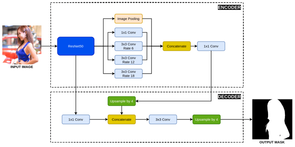
The network begins with a pre-trained ResNet50 as the encoder, which is followed by the ASPP. The ASPP consists of dilated convolution which helps to encode multi-scale contextual information. Next, it is followed by a bilinear upsampling by a factor of 4 and then concatenated with the low-level information from the encoder. After that, a few 3×3 convolutions is applied and again it is followed by a bilinear upsampling by a factor of 4. Finally at last we get the output mask.
model.py
At first, we import all the required layers, pre-trained ResNet50 and all the other classes and functions required.
import os
os.environ["TF_CPP_MIN_LOG_LEVEL"] = "2"

from tensorflow.keras.layers import Conv2D, BatchNormalization, Activation, MaxPool2D, Conv2DTranspose, Concatenate, Input

from tensorflow.keras.layers import AveragePooling2D, GlobalAveragePooling2D, UpSampling2D, Reshape, Dense

from tensorflow.keras.models import Model
from tensorflow.keras.applications import ResNet50
import tensorflow as tf
Now, we define the Squeeze and Excitation Network. It’s a channel-wise attention mechanism that helps improve the feature representation by suppressing irrelevant features and enhancing the important features.
def SqueezeAndExcite(inputs, ratio=8):
    init = inputs
    filters = init.shape[-1]
    se_shape = (1, 1, filters)

    se = GlobalAveragePooling2D()(init)
    se = Reshape(se_shape)(se)
    se = Dense(filters // ratio, activation='relu', kernel_initializer='he_normal', use_bias=False)(se)
    se = Dense(filters, activation='sigmoid', kernel_initializer='he_normal', use_bias=False)(se)
    x = init * se
    return x
Next, we define the Atrous Spatial Pyramid Pooling (ASPP).
def ASPP(inputs):
    """ Image Pooling """
    shape = inputs.shape
    y1 = AveragePooling2D(pool_size=(shape[1], shape[2]))(inputs)
    y1 = Conv2D(256, 1, padding="same", use_bias=False)(y1)
    y1 = BatchNormalization()(y1)
    y1 = Activation("relu")(y1)
    y1 = UpSampling2D((shape[1], shape[2]), interpolation="bilinear")(y1)

    """ 1x1 conv """
    y2 = Conv2D(256, 1, padding="same", use_bias=False)(inputs)
    y2 = BatchNormalization()(y2)
    y2 = Activation("relu")(y2)

    """ 3x3 conv rate=6 """
    y3 = Conv2D(256, 3, padding="same", use_bias=False, dilation_rate=6)(inputs)
    y3 = BatchNormalization()(y3)
    y3 = Activation("relu")(y3)

    """ 3x3 conv rate=12 """
    y4 = Conv2D(256, 3, padding="same", use_bias=False, dilation_rate=12)(inputs)
    y4 = BatchNormalization()(y4)
    y4 = Activation("relu")(y4)

    """ 3x3 conv rate=18 """
    y5 = Conv2D(256, 3, padding="same", use_bias=False, dilation_rate=18)(inputs)
    y5 = BatchNormalization()(y5)
    y5 = Activation("relu")(y5)

    y = Concatenate()([y1, y2, y3, y4, y5])
    y = Conv2D(256, 1, padding="same", use_bias=False)(y)
    y = BatchNormalization()(y)
    y = Activation("relu")(y)

    return y
Finally, we have our DeepLabV3+ architecture with Squeeze and Excitation attention mechanism.
def deeplabv3_plus(shape):
    """ Input """
    inputs = Input(shape)

    """ Encoder """
    encoder = ResNet50(weights="imagenet", include_top=False, input_tensor=inputs)

    image_features = encoder.get_layer("conv4_block6_out").output
    x_a = ASPP(image_features)
    x_a = UpSampling2D((4, 4), interpolation="bilinear")(x_a)

    x_b = encoder.get_layer("conv2_block2_out").output
    x_b = Conv2D(filters=48, kernel_size=1, padding='same', use_bias=False)(x_b)
    x_b = BatchNormalization()(x_b)
    x_b = Activation('relu')(x_b)

    x = Concatenate()([x_a, x_b])
    x = SqueezeAndExcite(x)

    x = Conv2D(filters=256, kernel_size=3, padding='same', use_bias=False)(x)
    x = BatchNormalization()(x)
    x = Activation('relu')(x)

    x = Conv2D(filters=256, kernel_size=3, padding='same', use_bias=False)(x)
    x = BatchNormalization()(x)
    x = Activation('relu')(x)
    x = SqueezeAndExcite(x)

    x = UpSampling2D((4, 4), interpolation="bilinear")(x)
    x = Conv2D(1, 1)(x)
    x = Activation("sigmoid")(x)

    model = Model(inputs, x)
    return model
Training the DeepLabV3+ architecture
Let’s have a recap and see what we have done till now. Till now, we have done the following:
- Data processing
- Loading the dataset.
- Split the dataset into training and testing.
- Applying data augmentation.
- Building the DeepLabV3+.
Now, we start training the DeepLabV3+ on the human image segmentation task.
train.py – First, we are going to import all the required classes and functions.
import os
os.environ["TF_CPP_MIN_LOG_LEVEL"] = "2"

import numpy as np
import cv2
from glob import glob
from sklearn.utils import shuffle
import tensorflow as tf
from tensorflow.keras.callbacks import ModelCheckpoint, CSVLogger, ReduceLROnPlateau, EarlyStopping, TensorBoard
from tensorflow.keras.optimizers import Adam
from tensorflow.keras.metrics import Recall, Precision
from model import deeplabv3_plus
from metrics import dice_loss, dice_coef, iou
Next, we have to define the two variables: H and W – height and width.
H = 512
W = 512
Here, we define the two functions:
- create_dir – It is used to create a directory.
- shuffling – It is used to shuffle the images and masks path list.
def create_dir(path):
    if not os.path.exists(path):
        os.makedirs(path)

def shuffling(x, y):
    x, y = shuffle(x, y, random_state=42)
    return x, y
Next, we are going to create a function called load_data. This function is used to load the dataset.
def load_data(path):
    x = sorted(glob(os.path.join(path, "image", "*png")))
    y = sorted(glob(os.path.join(path, "mask", "*png")))
    return x, y
Now, we are going to read the image and mask using the read_image and read_mask function respectively.
def read_image(path):
    path = path.decode()
    x = cv2.imread(path, cv2.IMREAD_COLOR)
    x = x/255.0
    x = x.astype(np.float32)
    return x

def read_mask(path):
    path = path.decode()
    x = cv2.imread(path, cv2.IMREAD_GRAYSCALE)
    x = x.astype(np.float32)
    x = np.expand_dims(x, axis=-1)
    return x
Now we will start building the input pipeline for training the DeepLabV3+ model on the dataset.
def tf_parse(x, y):
    def _parse(x, y):
        x = read_image(x)
        y = read_mask(y)
        return x, y

    x, y = tf.numpy_function(_parse, [x, y], [tf.float32, tf.float32])
    x.set_shape([H, W, 3])
    y.set_shape([H, W, 1])
    return x, y

def tf_dataset(X, Y, batch=2):
    dataset = tf.data.Dataset.from_tensor_slices((X, Y))
    dataset = dataset.map(tf_parse)
    dataset = dataset.batch(batch)
    dataset = dataset.prefetch(10)
    return dataset
Now, we are finished defining all the functions. The execution of the main program begins from here.
First, we are going to see the environment and create a directory called files to save all the data.
if __name__ == "__main__":
    np.random.seed(42)
    tf.random.set_seed(42)

    create_dir("files")
Next, we are going to define some hyperparameters.
    batch_size = 2
    lr = 1e-4
    num_epochs = 20
    model_path = os.path.join("files", "model.h5")
    csv_path = os.path.join("files", "data.csv")
Now we will load the training and validation/testing dataset and create the training and validation dataset pipeline.
    dataset_path = "new_data"
    train_path = os.path.join(dataset_path, "train")
    valid_path = os.path.join(dataset_path, "test")

    train_x, train_y = load_data(train_path)
    train_x, valid_y = shuffling(train_x, train_y)
    valid_x, valid_y = load_data(valid_path)

    print(f"Train: {len(train_x)} - {len(train_y)}")
    print(f"Valid: {len(valid_x)} - {len(valid_y)}")

    train_dataset = tf_dataset(train_x, train_y, batch=batch_size)
    valid_dataset = tf_dataset(valid_x, valid_y, batch=batch_size)
It’s now time to define our DeepLabV3+ model.
    model = deeplabv3_plus((H, W, 3))
    model.compile(loss=dice_loss, optimizer=Adam(lr), metrics=[dice_coef, iou, Recall(), Precision()])
Next, we define some callbacks, which are going to be used while training the model.
callbacks = [
        ModelCheckpoint(model_path, verbose=1, save_best_only=True),
        ReduceLROnPlateau(monitor='val_loss', factor=0.1, patience=5, min_lr=1e-7, verbose=1),
        CSVLogger(csv_path),
        TensorBoard(),
        EarlyStopping(monitor='val_loss', patience=20, restore_best_weights=False),
    ]
Now, finally, we start training the model using the fit function.
    model.fit(
        train_dataset,
        epochs=num_epochs,
        validation_data=valid_dataset,
        callbacks=callbacks
    )
Evaluation on the model
Now the model is successful trained. We are going to evaluate the model on different metrics to check its generalization performance. We are also going to save the predicted mask for visualization purposes.
eval.py – First, we are going to import all the required classes and functions.
import os
os.environ["TF_CPP_MIN_LOG_LEVEL"] = "2"

import numpy as np
import cv2
import pandas as pd
from glob import glob
from tqdm import tqdm
import tensorflow as tf
from tensorflow.keras.utils import CustomObjectScope
from sklearn.metrics import accuracy_score, f1_score, jaccard_score, precision_score, recall_score
from metrics import dice_loss, dice_coef, iou
from train import load_data, create_dir
Here, we are importing the accuracy_score, f1_score, jaccard_score, precision_score and recall_score functions from the sklearn library. These metrics are used to evaluate the model for its generalization capability.
Next, we have to define the two variables: H and W – height and width.
H = 512
W = 512
Here, we create a function called save_results. The function is used to concatenate the input image, ground truth mask and the predicted mask into a single image. Later, we save this single concatenated image.
The save_results function takes the following arguments:
- image – It is the numpy array representing the input image.
- mask – It is the numpy array representing the ground truth mask.
- y_pred – It is the numpy array representing the predicted mask.
- save_image_path – It is the path where the concatenated image needs to be saved.
def save_results(image, mask, y_pred, save_image_path):
    line = np.ones((H, 10, 3)) * 128

    mask = np.expand_dims(mask, axis=-1)    ## (512, 512, 1)
    mask = np.concatenate([mask, mask, mask], axis=-1)  ## (512, 512, 3)
    mask = mask * 255

    y_pred = np.expand_dims(y_pred, axis=-1)    ## (512, 512, 1)
    y_pred = np.concatenate([y_pred, y_pred, y_pred], axis=-1)  ## (512, 512, 3)

    masked_image = image * y_pred
    y_pred = y_pred * 255

    cat_images = np.concatenate([image, line, mask, line, y_pred, line, masked_image], axis=1)
    cv2.imwrite(save_image_path, cat_images)
Now we start with the execution of the program.
if __name__ == "__main__":
    np.random.seed(42)
    tf.random.set_seed(42)

   create_dir("results")
First, we seed the environment with the same seed number that is used in the training part. Next, we create a directory to save the results.
Next, we load the trained DeepLabV3+ model.
    with CustomObjectScope({'iou': iou, 'dice_coef': dice_coef, 'dice_loss': dice_loss}):
        model = tf.keras.models.load_model("files/model.h5")
Now we load the test dataset images and masks into the test_x and test_y variables respectively.
    dataset_path = "new_data"
    valid_path = os.path.join(dataset_path, "test")
    test_x, test_y = load_data(valid_path)
    print(f"Test: {len(test_x)} - {len(test_y)}")
We would now loop over the test images and masks i.e., test_x and test_y.
    SCORE = []
    for x, y in tqdm(zip(test_x, test_y), total=len(test_x)):
        name = x.split("/")[-1].split(".")[0]
Next, we would extract the name from the image path i.e., x variable. We would use this name while saving the concatenated image.
Now, we are going to read the image and mask.
        image = cv2.imread(x, cv2.IMREAD_COLOR)
        x = image/255.0
        x = np.expand_dims(x, axis=0)

        mask = cv2.imread(y, cv2.IMREAD_GRAYSCALE)
Now, we use the image and make a prediction and get the predicted mask in the y_pred variable.
        y_pred = model.predict(x)[0]
        y_pred = np.squeeze(y_pred, axis=-1)
        y_pred = y_pred > 0.5
        y_pred = y_pred.astype(np.int32)
The y_pred contains the pixel value between 0 and 1. So, we apply a threshold value of 0.5 to convert the y_pred mask pixel values into 0 and 1.
Here the pixel value 0 represents the background class and the 1 represents the foreground class or the person/people class.
        save_image_path = f"results/{name}.png"
        save_results(image, mask, y_pred, save_image_path)
Now we concatenate all the images and save them in the path provided by the save_image_path variable.
Next, we are going to calculate the performance by using the various metrics function.
        mask = mask.flatten()
        y_pred = y_pred.flatten()

        """ Calculating the metrics values """
        acc_value = accuracy_score(mask, y_pred)
        f1_value = f1_score(mask, y_pred, labels=[0, 1], average="binary")
        jac_value = jaccard_score(mask, y_pred, labels=[0, 1], average="binary")
        recall_value = recall_score(mask, y_pred, labels=[0, 1], average="binary")
        precision_value = precision_score(mask, y_pred, labels=[0, 1], average="binary")
        SCORE.append([name, acc_value, f1_value, jac_value, recall_value, precision_value])
We append all the metrics scores in the SCORE variable along with the name of the image.
    score = [s[1:]for s in SCORE]
    score = np.mean(score, axis=0)
    print(f"Accuracy: {score[0]:0.5f}")
    print(f"F1: {score[1]:0.5f}")
    print(f"Jaccard: {score[2]:0.5f}")
    print(f"Recall: {score[3]:0.5f}")
    print(f"Precision: {score[4]:0.5f}")

    df = pd.DataFrame(SCORE, columns=["Image", "Accuracy", "F1", "Jaccard", "Recall", "Precision"])
    df.to_csv("files/score.csv")
Now, we get the final mean scores for all metrics and we save all the individual scores in a CSV file for better analysis.
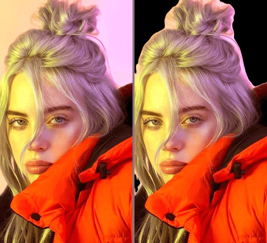
Prediction on images from internet.
To check the generalization of the model, we have downloaded some images from https://wallpapercave.com. We have made predictions on these images and overlay the predicted mask on the image.
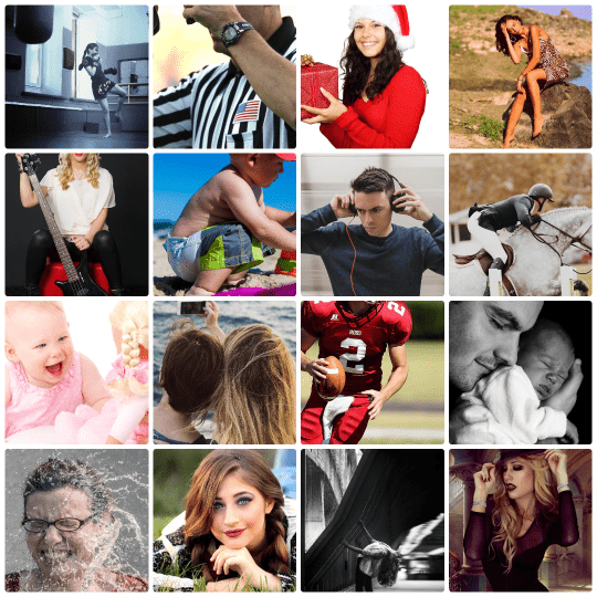
Collecting images from internet.
I have to download the images from this link: https://wallpapercave.com/pretty-people-wallpapers. To download these images I have used a Google Extension called Fatkun – Batch Download Image.
Predicting mask
predict.py – Importing
import os
os.environ["TF_CPP_MIN_LOG_LEVEL"] = "2"

import numpy as np
import cv2
import pandas as pd
from glob import glob
from tqdm import tqdm
import tensorflow as tf
from tensorflow.keras.utils import CustomObjectScope
from metrics import dice_loss, dice_coef, iou
from train import create_dir
Defining the height and width.
H = 512
W = 512
Now, we are going to seed the environment, then create a directory to save the mask. Next, we load the trained DeepLabV3+ and the images.
if __name__ == "__main__":
    np.random.seed(42)
    tf.random.set_seed(42)

    create_dir("test_images/mask")

    with CustomObjectScope({'iou': iou, 'dice_coef': dice_coef, 'dice_loss': dice_loss}):
        model = tf.keras.models.load_model("files/model.h5")

    data_x = glob("test_images/image/*")
We would now loop over the images and extract the names from the image path.
    for path in tqdm(data_x, total=len(data_x)):
        name = path.split("/")[-1].split(".")[0]
Now, we read the image and process it.
        image = cv2.imread(path, cv2.IMREAD_COLOR)
        h, w, _ = image.shape
        x = cv2.resize(image, (W, H))
        x = x/255.0
        x = x.astype(np.float32)
        x = np.expand_dims(x, axis=0)
Now we are going to make predicted the mask for the input image.
y = model.predict(x)[0]
y = cv2.resize(y, (w, h))
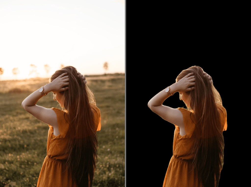
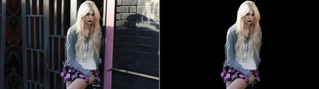
y = np.expand_dims(y, axis=-1)Finally, we overlay the binary mask over the input image and save them.
        masked_image = image * y
        line = np.ones((h, 10, 3)) * 128
        cat_images = np.concatenate([image, line, masked_image], axis=1)
        cv2.imwrite(f"test_images/mask/{name}.png", cat_images)
Here are some of the images samples. The first is the original image and the second is the overlay image.
Conclusion
I hope you learned something new from this article. Please make sure that you leave a comment. You can also subscribe to our YouTube channel.
IDIOT DEVELOPER – https://www.youtube.com/c/IdiotDeveloper/?sub_confirmation=1

Thanks for the sharing of DeeplabV3 architecure. I met a problem in traning my own data. The loss is negative, both dice_coef and iou are big than 1, sometimes “iou” is big than 20. I have searched all the post and blogs online, but no one suggestion can fix my problem, could you please help me with this, thank you .
IOU and Dice cofficient are big than 1, how to solve these problem, thanks