
In this tutorial, we are going to work on UNet segmentation and use it for biomedical image segmentation tasks. This time we are going to use pre-trained MobileNetV2 as the encoder for the UNet architecture. We are going to integrate the pre-trained MobileNetV2 with the UNet and have an efficient network architecture. The MobileNetV2 is trained on the ImageNet dataset, which is one of the largest and most popular dataset commonly used.
In this tutorial, we are going to learn:
- What is UNet
- What is MobileNetV2
- Advantages of using MobileNetV2 as an encoder.
- Dataset
- Implementation
- Improve the Results
- Conclusion
What is UNet
U-Net is a convolutional neural network that was developed for biomedical image segmentation at the Computer Science Department of the University of Freiburg, Germany. The network is based on the fully convolutional network and its architecture was modified and extended to work with fewer training images and to yield more precise segmentations.
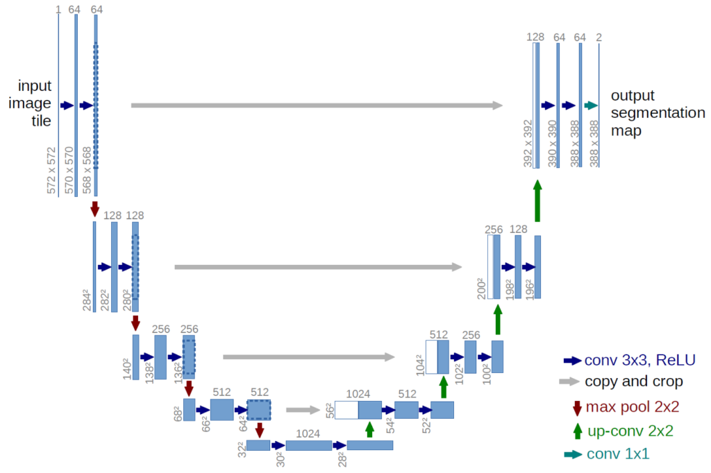
Paper: U-Net: Convolutional Networks for Biomedical Image Segmentation
For more:
What is MobileNetV2
MobileNetV2 is an architecture that is optimized for mobile devices. It improves the state of the art performance of mobile models on multiple tasks and benchmarks as well as across a spectrum of different model sizes.
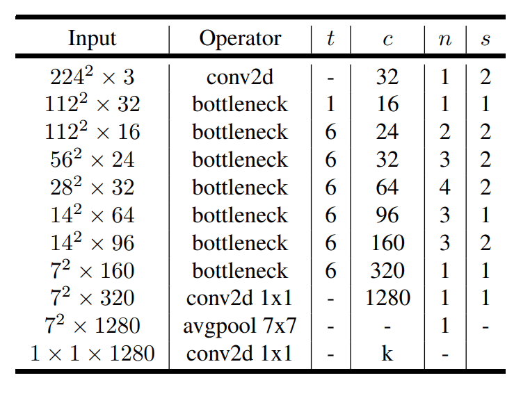
Paper: MobileNetV2: Inverted Residuals and Linear Bottlenecks
The MobileNetV2 is used for the encoder/downsampling path of the U-Net (the left half of the U)
Advantages of using MobileNetV2 as an Encoder
- MobileNetV2 has less parameters, due to which it is easy to train.
- Using a pre-trained encoder helps the model to converge much faster in comparison to the non-pretrained model.
- A pre-trained encoder helps the model to achieve high performance as compared to a non pre-trained model.
Dataset
For this tutorial, we are using CVC-612 or CVC-ClinicDB which is a polyp segmentation dataset. You can download the dataset from here or directly from Dropbox.
Implementation
The UNet architecture with pre-trained MobileNetV2 as the encoder is implemented in python 3.8 using TensorFlow 2.2.0.
import os
import numpy as np
import cv2
from glob import glob
import tensorflow as tf
import matplotlib.pyplot as plt
from sklearn.model_selection import train_test_split

from tensorflow.keras.layers import Conv2D, Activation, BatchNormalization
from tensorflow.keras.layers import UpSampling2D, Input, Concatenate
from tensorflow.keras.models import Model
from tensorflow.keras.applications import MobileNetV2
from tensorflow.keras.callbacks import EarlyStopping, ReduceLROnPlateau
from tensorflow.keras.metrics import Recall, Precision
from tensorflow.keras import backend as K
Here, we import all the necessary libraries and functions required for the implementation for the UNet in TensorFlow.
np.random.seed(42)
tf.random.set_seed(42)
Next, we set the set the seed value of the NumPy and TensorFlow. Seeding helps to set the randomness of the environment and also helps to make the results reproducible.
IMAGE_SIZE = 256
EPOCHS = 30
BATCH = 8
LR = 1e-4
PATH = "CVC-612/"
Here, we set some of the hyperparameters that are used while training the UNet architecture,
def load_data(path, split=0.1):
    images = sorted(glob(os.path.join(path, "images/*")))
    masks = sorted(glob(os.path.join(path, "masks/*")))

    total_size = len(images)
    valid_size = int(split * total_size)
    test_size = int(split * total_size)

    train_x, valid_x = train_test_split(images, test_size=valid_size, random_state=42)
    train_y, valid_y = train_test_split(masks, test_size=valid_size, random_state=42)

    train_x, test_x = train_test_split(train_x, test_size=test_size, random_state=42)
    train_y, test_y = train_test_split(train_y, test_size=test_size, random_state=42)

    return (train_x, train_y), (valid_x, valid_y), (test_x, test_y)
The load_data function takes the path of the dataset, which we have already specified above in the hyperparameter section. This function loads the images and masks, split them into training, validation and testing dataset using 80-10-10 ratio.
def read_image(path):
    path = path.decode()
    x = cv2.imread(path, cv2.IMREAD_COLOR)
    x = cv2.resize(x, (IMAGE_SIZE, IMAGE_SIZE))
    x = x/255.0
    return x

def read_mask(path):
    path = path.decode()
    x = cv2.imread(path, cv2.IMREAD_GRAYSCALE)
    x = cv2.resize(x, (IMAGE_SIZE, IMAGE_SIZE))
    x = x/255.0
    x = np.expand_dims(x, axis=-1)
    return x
Here, we write two functions: read_image and read_mask. Both these functions read the image from the given path, resize them to 256 x 256, normalize them by dividing with 255.0 and then returning a RGB image and a grayscale mask respectively.
def tf_parse(x, y):
    def _parse(x, y):
        x = read_image(x)
        y = read_mask(y)
        return x, y

    x, y = tf.numpy_function(_parse, [x, y], [tf.float64, tf.float64])
    x.set_shape([IMAGE_SIZE, IMAGE_SIZE, 3])
    y.set_shape([IMAGE_SIZE, IMAGE_SIZE, 1])
    return x, y

def tf_dataset(x, y, batch=8):
    dataset = tf.data.Dataset.from_tensor_slices((x, y))
    dataset = dataset.map(tf_parse)
    dataset = dataset.batch(batch)
    dataset = dataset.repeat()
    return dataset
The above two functions tf_parse and tf_dataset are used to build the dataset pipeline.
The tf_dataset function create a tf.data pipeline which takes a list of images, masks paths and the batch size. The tf_parse function parses a single image and mask path.
def read_and_rgb(x):
    x = cv2.imread(x)
    x = cv2.cvtColor(x, cv2.COLOR_BGR2RGB)
    return x
The read_and_rgb function is used to take the image path, read it and convert to the RGB formart from the BGR format.
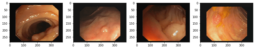
fig = plt.figure(figsize=(15, 15))
a = fig.add_subplot(1, 4, 1)
imgplot = plt.imshow(read_and_rgb(train_x[0]))

a = fig.add_subplot(1, 4, 2)
imgplot = plt.imshow(read_and_rgb(train_x[1]))
imgplot.set_clim(0.0, 0.7)

a = fig.add_subplot(1, 4, 3)
imgplot = plt.imshow(read_and_rgb(train_x[2]))
imgplot.set_clim(0.0, 1.4)

a = fig.add_subplot(1, 4, 4)
imgplot = plt.imshow(read_and_rgb(train_x[3]))
imgplot.set_clim(0.0, 2.1)

fig = plt.figure(figsize=(15, 15))
a = fig.add_subplot(1, 4, 1)
imgplot = plt.imshow(read_and_rgb(train_y[0]))

a = fig.add_subplot(1, 4, 2)
imgplot = plt.imshow(read_and_rgb(train_y[1]))
imgplot.set_clim(0.0, 0.7)

a = fig.add_subplot(1, 4, 3)
imgplot = plt.imshow(read_and_rgb(train_y[2]))
imgplot.set_clim(0.0, 1.4)

a = fig.add_subplot(1, 4, 4)
imgplot = plt.imshow(read_and_rgb(train_y[3]))
imgplot.set_clim(0.0, 1.4)
The above lines of code are used for the visualization of the images and their respective masks.

def model():
    inputs = Input(shape=(IMAGE_SIZE, IMAGE_SIZE, 3), name="input_image")

    encoder = MobileNetV2(input_tensor=inputs, weights="imagenet", include_top=False, alpha=0.35)
    skip_connection_names = ["input_image", "block_1_expand_relu", "block_3_expand_relu", "block_6_expand_relu"]
    encoder_output = encoder.get_layer("block_13_expand_relu").output

    f = [16, 32, 48, 64]
    x = encoder_output
    for i in range(1, len(skip_connection_names)+1, 1):
        x_skip = encoder.get_layer(skip_connection_names[-i]).output
        x = UpSampling2D((2, 2))(x)
        x = Concatenate()([x, x_skip])

        x = Conv2D(f[-i], (3, 3), padding="same")(x)
        x = BatchNormalization()(x)
        x = Activation("relu")(x)

        x = Conv2D(f[-i], (3, 3), padding="same")(x)
        x = BatchNormalization()(x)
        x = Activation("relu")(x)

    x = Conv2D(1, (1, 1), padding="same")(x)
    x = Activation("sigmoid")(x)

    model = Model(inputs, x)
    return model
The model function is used to build the architecture for the UNet with pre-trained MobileNetV2.
smooth = 1e-15
def dice_coef(y_true, y_pred):
    y_true = tf.keras.layers.Flatten()(y_true)
    y_pred = tf.keras.layers.Flatten()(y_pred)
    intersection = tf.reduce_sum(y_true * y_pred)
    return (2. * intersection + smooth) / (tf.reduce_sum(y_true) + tf.reduce_sum(y_pred) + smooth)

def dice_loss(y_true, y_pred):
    return 1.0 - dice_coef(y_true, y_pred)
Here, we define the dice coefficient which is used as the metric to measure the performance and the dice coefficient loss.
train_dataset = tf_dataset(train_x, train_y, batch=BATCH)
valid_dataset = tf_dataset(valid_x, valid_y, batch=BATCH)
The training and validation input dataset pipelines are build with the tf_dataset function. The tf_dataset take the images paths and masks paths as a list. It also takes the batch size.
model = model()
opt = tf.keras.optimizers.Nadam(LR)
metrics = [dice_coef, Recall(), Precision()]
model.compile(loss=dice_loss, optimizer=opt, metrics=metrics)
Here, we call the model function to build the UNet with MobileNetV2 as pre-trained encoder. To train the architecture, we use Adam optimizer with dice coefficient loss.
callbacks = [
    ReduceLROnPlateau(monitor='val_loss', factor=0.1, patience=4),
    EarlyStopping(monitor='val_loss', patience=10, restore_best_weights=False)
]
The callbacks are used while training a network. We used two callbacks:
- ReduceLROnPlateau: Reduce learning when a monitored metric has stopped improving.
- EarlyStopping: Stop training when a monitored metric has stopped improving.
train_steps = len(train_x)//BATCH
valid_steps = len(valid_x)//BATCH

if len(train_x) % BATCH != 0:
    train_steps += 1
if len(valid_x) % BATCH != 0:
    valid_steps += 1
First we define the training and validation steps, which define the number of batches in an epoch.
model.fit(
    train_dataset,
    validation_data=valid_dataset,
    epochs=EPOCHS,
    steps_per_epoch=train_steps,
    validation_steps=valid_steps,
    callbacks=callbacks
)
The fit function is used for training a UNet on the polyp segmentation dataset.
test_dataset = tf_dataset(test_x, test_y, batch=BATCH)

test_steps = (len(test_x)//BATCH)
if len(test_x) % BATCH != 0:
    test_steps += 1

model.evaluate(test_dataset, steps=test_steps)
The above line of code are used for evaluating the trained model on the test dataset.
First, we use the tf_dataset to create the test dataset pipeline for evaluation. After that, we define the test steps and al last we use the evaluate function to get the test dataset results.
8/8 [==============================] - 0s 27ms/step - loss: 0.2378 - dice_coef: 0.7656 - recall: 0.7618 - precision: 0.8595
[0.23775120079517365,  0.7655861377716064,  0.7617509961128235,  0.8594527840614319]
def read_image(path):
    x = cv2.imread(path, cv2.IMREAD_COLOR)
    x = cv2.cvtColor(x, cv2.COLOR_BGR2RGB)
    x = cv2.resize(x, (IMAGE_SIZE, IMAGE_SIZE))
    x = x/255.0
    return x

def read_mask(path):
    x = cv2.imread(path, cv2.IMREAD_GRAYSCALE)
    x = cv2.resize(x, (IMAGE_SIZE, IMAGE_SIZE))
    x = np.expand_dims(x, axis=-1)
    x = x/255.0
    return x
The above functions are same as we define above. They are used to read the image and mask from the given path.
def mask_parse(mask):
mask = np.squeeze(mask)
mask = [mask, mask, mask]
mask = np.transpose(mask, (1, 2, 0))
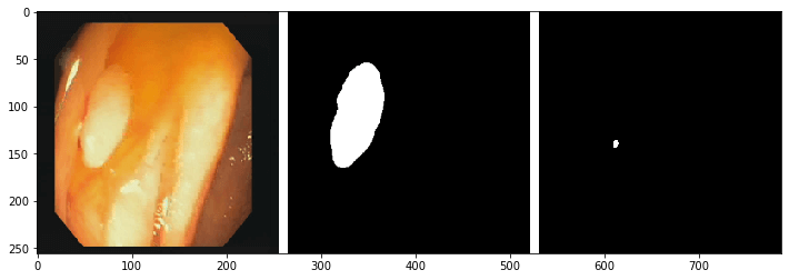
return maskThe mask_parse function is used while joining the input image, ground truth mask and the predicted mask to form a single image.
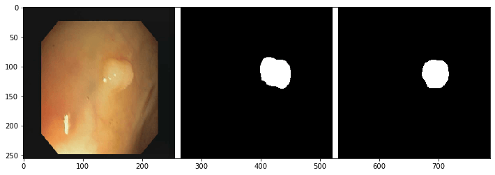
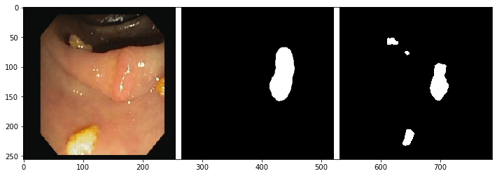
for i, (x, y) in enumerate(zip(test_x[:10], test_y[:10])):
    x = read_image(x)
    y = read_mask(y)
    y_pred = model.predict(np.expand_dims(x, axis=0))[0] > 0.5
    h, w, _ = x.shape
    white_line = np.ones((h, 10, 3))

    all_images = [
        x, white_line,
        mask_parse(y), white_line,
        mask_parse(y_pred)
    ]
    image = np.concatenate(all_images, axis=1)

    fig = plt.figure(figsize=(12, 12))
    a = fig.add_subplot(1, 1, 1)
    imgplot = plt.imshow(image)
In the above line of code takes the test dataset image, makes the prediction on it and then concatenate all the three images i.e., input image, ground truth and the predicted mask
| INPUT IMAGE | GROUND TRUTH | PREDICTED MASK |
Improve the Results
- Use data augmentation
- Use other pretrained encoder
- Use a different decoder or different blocks in the decoder.
Conclusion
This is all about UNet with pre-trained MobileNetV2. I hope that you find this tutorial useful and make sure that you also subscribe to my YouTube channel.


Dear Nikhil,
I notice when I ran the below cell in the code
model = model()
immediately it occupied 22Gb of GPU is it normal?
Thank you for your support
Yeah. it is normal.