In this article, we will implement the UNet 3+ architecture using TensorFlow. UNet 3+ extends the classic UNet and UNet++ architecture incorporating full skip connections. We will delve into each block of the UNet 3+ architecture, explaining how they work and how they contribute to improving the model’s performance. Understanding these blocks will provide insights into the mechanisms behind UNet 3+ and how it effectively handles tasks such as image segmentation or other pixel-wise prediction tasks.
RESEARCH PAPER: UNET 3+: A FULL-SCALE CONNECTED UNET FOR MEDICAL IMAGE SEGMENTATION
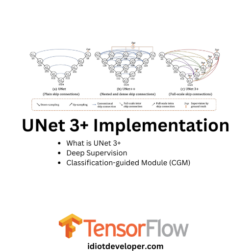
What is UNet 3+?
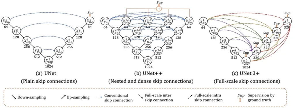
UNet 3+ is a U-shape encoder-decoder architecture built upon the foundation of its predecessors, i.e., UNet and UNet++. It aims to capture both fine-grained details and coarse-grained semantics from full scales. The paper highlights the re-design of inter and intra-connections between the encoder and the decoder, providing a more comprehensive understanding of organ structures.
Additionally, a hybrid loss function contributes to accurate segmentation, especially for organs appearing at varying scales, while reducing network parameters to improve computational efficiency.
READ MORE: [Paper Summary] UNet 3+: A Full-Scale Connected UNET For Medical Image Segmentation
UNet 3+ Varients
It consists of three variants:
- Simple UNet 3+
- UNet 3+ with Deep Supervision
- UNet 3+ with Deep Supervision and Classification-guided Module (CGM)
Simple UNet 3+
We will begin with implementing the basic UNet 3+, which consists of a simple encoder-decoder structure. It takes an input image and predicts a segmentation mask. Later, we will add other components, such as the Deep Supervision and Classification-guided Module (CGM), to build the remaining variants.
First, we will import the TensorFlow library.
Import Library
import tensorflow as tf
import tensorflow.keras.layers as L
Convolution Block
The conv_block function is the fundamental building block of the UNet 3+ and will be utilized throughout the whole architecture.
def conv_block(x, num_filters, act=True):
    x = L.Conv2D(num_filters, kernel_size=3, padding="same")(x)

    if act == True:
        x = L.BatchNormalization()(x)
        x = L.Activation("relu")(x)

    return x
The conv_block function takes the following arguments:
- x – It is the input feature map, which will be passed through the convolution layer.
- num_filters – These are the number of output feature channels.
- act – It is a boolean variable; by default, its value is True.
If the act is True, then the output of the convolution layer will pass through the batch normalization and ReLU activation function.
Encoder Block
The encoder_block is used to extract and encode features from the input image.
def encoder_block(x, num_filters):
    x = conv_block(x, num_filters)
    x = conv_block(x, num_filters)

    p = L.MaxPool2D((2, 2))(x)
    return x, p
The encoder_block consists of two conv_block, followed by a 2×2 max-pooling layer. The convolution layers play a crucial role in feature extraction by applying filters to the input image, which helps capture spatial patterns and details. The max-pooling layer downsamples the feature maps, reducing their spatial dimensions while retaining the most important information.
The encoder_block returns two values, x, and p. Here, x represents the output of conv_block, which is utilized in the decoder part as a skip connection. The p represents the output of the max-pooling layer.
Now, we began with the Simple UNet 3+.
Simple UNet 3+
The unet3plus function takes the input shape and the number of classes present in the dataset. Next, it is followed by four encoder blocks, and we have bottleneck (bridge) layers.
def unet3plus(input_shape, num_classes=1):
    """ Inputs """
    inputs = L.Input(input_shape, name="input_layer")

    """ Encoder """
    e1, p1 = encoder_block(inputs, 64)
    e2, p2 = encoder_block(p1, 128)
    e3, p3 = encoder_block(p2, 256)
    e4, p4 = encoder_block(p3, 512)

    """ Bottleneck """
    e5 = conv_block(p4, 1024)
    e5 = conv_block(e5, 1024)
Now, we move on to the decoder. The UNet 3+ has four decoder blocks, each utilizing all the features from the encoder and bottleneck part of the network.
Additionally, features from the previous decoder blocks are also used. This innovative approach captures fine-grained details and coarse-grained semantics in full scales, enhancing the model’s position awareness and boundary definition.
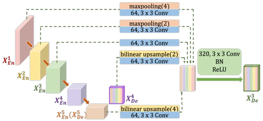
Let us now understand and implement the decoder 4.
    """ Decoder 4 """
    e1_d4 = L.MaxPool2D((8, 8))(e1)
    e1_d4 = conv_block(e1_d4, 64)

    e2_d4 = L.MaxPool2D((4, 4))(e2)
    e2_d4 = conv_block(e2_d4, 64)

    e3_d4 = L.MaxPool2D((2, 2))(e3)
    e3_d4 = conv_block(e3_d4, 64)

    e4_d4 = conv_block(e4, 64)

    e5_d4 = L.UpSampling2D((2, 2), interpolation="bilinear")(e5)
    e5_d4 = conv_block(e5_d4, 64)

    d4 = L.Concatenate()([e1_d4, e2_d4, e3_d4, e4_d4, e5_d4])
    d4 = conv_block(d4, 64*5)
The above code takes multi-scale feature maps from the encoder and bottleneck layers— e1, e2, e3, e4, and e5. Proper max-pooling and bilinear upsampling layers ensure that all these feature maps have the same height and width. Each is followed by a conv_block with 64 output feature channels.
Next, we concatenate all these features and pass them again through a conv_block, which acts as the output of the decoder block.
Let’s delve into the remaining decoder blocks. One subtle difference between the first decoder block we discussed and the subsequent three decoder blocks is that we leverage features from previous decoders, aiding in more effective feature propagation across the network.
   """ Decoder 3 """
    e1_d3 = L.MaxPool2D((4, 4))(e1)
    e1_d3 = conv_block(e1_d3, 64)

    e2_d3 = L.MaxPool2D((2, 2))(e2)
    e2_d3 = conv_block(e2_d3, 64)

    e3_d3 = conv_block(e3, 64)

    d4_d3 = L.UpSampling2D((2, 2), interpolation="bilinear")(d4)
    d4_d3 = conv_block(d4_d3, 64)

    e5_d3 = L.UpSampling2D((4, 4), interpolation="bilinear")(e5)
    e5_d3 = conv_block(e5_d3, 64)

    d3 = L.Concatenate()([e1_d3, e2_d3, e3_d3, d4_d3, e5_d3])
    d3 = conv_block(d3, 64*5)

    """ Decoder 2 """
    e1_d2 = L.MaxPool2D((2, 2))(e1)
    e1_d2 = conv_block(e1_d2, 64)

    e2_d2 = conv_block(e2, 64)

    d3_d2 = L.UpSampling2D((2, 2), interpolation="bilinear")(d3)
    d3_d2 = conv_block(d3_d2, 64)

    d4_d2 = L.UpSampling2D((4, 4), interpolation="bilinear")(d4)
    d4_d2 = conv_block(d4_d2, 64)

    e5_d2 = L.UpSampling2D((8, 8), interpolation="bilinear")(e5)
    e5_d2 = conv_block(e5_d2, 64)

    d2 = L.Concatenate()([e1_d2, e2_d2, d3_d2, d4_d2, e5_d2])
    d2 = conv_block(d2, 64*5)

    """ Decoder 1 """
    e1_d1 = conv_block(e1, 64)

    d2_d1 = L.UpSampling2D((2, 2), interpolation="bilinear")(d2)
    d2_d1 = conv_block(d2_d1, 64)

    d3_d1 = L.UpSampling2D((4, 4), interpolation="bilinear")(d3)
    d3_d1 = conv_block(d3_d1, 64)

    d4_d1 = L.UpSampling2D((8, 8), interpolation="bilinear")(d4)
    d4_d1 = conv_block(d4_d1, 64)

    e5_d1 = L.UpSampling2D((16, 16), interpolation="bilinear")(e5)
    e5_d1 = conv_block(e5_d1, 64)

    d1 = L.Concatenate()([e1_d1, d2_d1, d3_d1, d4_d1, e5_d1])
    d1 = conv_block(d1, 64*5)
Now, we add a simple 1×1 convolution layer with the number of classes as the number of output channels to predict the segmentation mask, followed by an activation function.
    """ Output """
    y1 = L.Conv2D(num_classes, kernel_size=3, padding="same")(d1)
    y1 = L.Activation("sigmoid")(y1)
    outputs = [y1]

    model = tf.keras.Model(inputs, outputs)
    return model
We have finally built our simple UNet 3+ model. Now, let’s add Deep Supervision into it.
UNet 3+ with Deep Supervision
Deep supervision is a training technique used in deep learning architectures, particularly in models with multiple layers or branches. It involves adding auxiliary classifiers or intermediate supervision points at various depths within the network. These auxiliary classifiers are trained alongside the main network output and provide additional gradient signals during backpropagation.
Deep supervision addresses the vanishing gradient problem, where gradients diminish as they propagate through many layers in a deep neural network. By introducing intermediate supervision, the model receives gradient feedback at multiple points during training, which can help stabilize training, accelerate convergence, and improve the overall performance of the network by encouraging the learning of more meaningful representations at different levels of abstraction.
Next, we’ll incorporate additional 1×1 convolution layers into the output of each decoder block and the bottleneck layer.
    """ Deep Supervision """
    if deep_sup == True:
        y1 = L.Conv2D(num_classes, kernel_size=3, padding="same")(d1)
        y1 = L.Activation("sigmoid")(y1)

        y2 = L.Conv2D(num_classes, kernel_size=3, padding="same")(d2)
        y2 = L.UpSampling2D((2, 2), interpolation="bilinear")(y2)
        y2 = L.Activation("sigmoid")(y2)

        y3 = L.Conv2D(num_classes, kernel_size=1, padding="same")(d3)
        y3 = L.UpSampling2D((4, 4), interpolation="bilinear")(y3)
        y3 = L.Activation("sigmoid")(y3)

        y4 = L.Conv2D(num_classes, kernel_size=1, padding="same")(d4)
        y4 = L.UpSampling2D((8, 8), interpolation="bilinear")(y4)
        y4 = L.Activation("sigmoid")(y4)

        y5 = L.Conv2D(num_classes, kernel_size=1, padding="same")(e5)
        y5 = L.UpSampling2D((16, 16), interpolation="bilinear")(y5)
        y5 = L.Activation("sigmoid")(y5)

        outputs = [y1, y2, y3, y4, y5]

    else:
        y1 = L.Conv2D(num_classes, kernel_size=1, padding="same")(d1)
        y1 = L.Activation("sigmoid")(y1)
        outputs = [y1]

    model = tf.keras.Model(inputs, outputs)
    return model
Complete Code
def unet3plus(input_shape, num_classes=1, deep_sup=True):
    """ Inputs """
    inputs = L.Input(input_shape, name="input_layer")

    """ Encoder """
    e1, p1 = encoder_block(inputs, 64)
    e2, p2 = encoder_block(p1, 128)
    e3, p3 = encoder_block(p2, 256)
    e4, p4 = encoder_block(p3, 512)

    """ Bottleneck """
    e5 = conv_block(p4, 1024)
    e5 = conv_block(e5, 1024)

    """ Decoder 4 """
    e1_d4 = L.MaxPool2D((8, 8))(e1)
    e1_d4 = conv_block(e1_d4, 64)

    e2_d4 = L.MaxPool2D((4, 4))(e2)
    e2_d4 = conv_block(e2_d4, 64)

    e3_d4 = L.MaxPool2D((2, 2))(e3)
    e3_d4 = conv_block(e3_d4, 64)

    e4_d4 = conv_block(e4, 64)

    e5_d4 = L.UpSampling2D((2, 2), interpolation="bilinear")(e5)
    e5_d4 = conv_block(e5_d4, 64)

    d4 = L.Concatenate()([e1_d4, e2_d4, e3_d4, e4_d4, e5_d4])
    d4 = conv_block(d4, 64*5)

    """ Decoder 3 """
    e1_d3 = L.MaxPool2D((4, 4))(e1)
    e1_d3 = conv_block(e1_d3, 64)

    e2_d3 = L.MaxPool2D((2, 2))(e2)
    e2_d3 = conv_block(e2_d3, 64)

    e3_d3 = conv_block(e3, 64)

    d4_d3 = L.UpSampling2D((2, 2), interpolation="bilinear")(d4)
    d4_d3 = conv_block(d4_d3, 64)

    e5_d3 = L.UpSampling2D((4, 4), interpolation="bilinear")(e5)
    e5_d3 = conv_block(e5_d3, 64)

    d3 = L.Concatenate()([e1_d3, e2_d3, e3_d3, d4_d3, e5_d3])
    d3 = conv_block(d3, 64*5)

    """ Decoder 2 """
    e1_d2 = L.MaxPool2D((2, 2))(e1)
    e1_d2 = conv_block(e1_d2, 64)

    e2_d2 = conv_block(e2, 64)

    d3_d2 = L.UpSampling2D((2, 2), interpolation="bilinear")(d3)
    d3_d2 = conv_block(d3_d2, 64)

    d4_d2 = L.UpSampling2D((4, 4), interpolation="bilinear")(d4)
    d4_d2 = conv_block(d4_d2, 64)

    e5_d2 = L.UpSampling2D((8, 8), interpolation="bilinear")(e5)
    e5_d2 = conv_block(e5_d2, 64)

    d2 = L.Concatenate()([e1_d2, e2_d2, d3_d2, d4_d2, e5_d2])
    d2 = conv_block(d2, 64*5)

    """ Decoder 1 """
    e1_d1 = conv_block(e1, 64)

    d2_d1 = L.UpSampling2D((2, 2), interpolation="bilinear")(d2)
    d2_d1 = conv_block(d2_d1, 64)

    d3_d1 = L.UpSampling2D((4, 4), interpolation="bilinear")(d3)
    d3_d1 = conv_block(d3_d1, 64)

    d4_d1 = L.UpSampling2D((8, 8), interpolation="bilinear")(d4)
    d4_d1 = conv_block(d4_d1, 64)

    e5_d1 = L.UpSampling2D((16, 16), interpolation="bilinear")(e5)
    e5_d1 = conv_block(e5_d1, 64)

    d1 = L.Concatenate()([e1_d1, d2_d1, d3_d1, d4_d1, e5_d1])
    d1 = conv_block(d1, 64*5)

    """ Deep Supervision """
    if deep_sup == True:
        y1 = L.Conv2D(num_classes, kernel_size=3, padding="same")(d1)
        y1 = L.Activation("sigmoid")(y1)

        y2 = L.Conv2D(num_classes, kernel_size=3, padding="same")(d2)
        y2 = L.UpSampling2D((2, 2), interpolation="bilinear")(y2)
        y2 = L.Activation("sigmoid")(y2)

        y3 = L.Conv2D(num_classes, kernel_size=1, padding="same")(d3)
        y3 = L.UpSampling2D((4, 4), interpolation="bilinear")(y3)
        y3 = L.Activation("sigmoid")(y3)

        y4 = L.Conv2D(num_classes, kernel_size=1, padding="same")(d4)
        y4 = L.UpSampling2D((8, 8), interpolation="bilinear")(y4)
        y4 = L.Activation("sigmoid")(y4)

        y5 = L.Conv2D(num_classes, kernel_size=1, padding="same")(e5)
        y5 = L.UpSampling2D((16, 16), interpolation="bilinear")(y5)
        y5 = L.Activation("sigmoid")(y5)

        outputs = [y1, y2, y3, y4, y5]

    else:
        y1 = L.Conv2D(num_classes, kernel_size=1, padding="same")(d1)
        y1 = L.Activation("sigmoid")(y1)
        outputs = [y1]

    model = tf.keras.Model(inputs, outputs)
    return model
UNet 3+ with Deep Supervision and Classification-guided Module (CGM)
We will add Deep Supervision and Classification-guided Module (CGM) to the Simple UNet 3+ to enhance its feature propagation and boost performance.
To tackle false positives, particularly in non-organ images, UNet 3+ introduces a classification-guided module. This involves an additional classification task to predict organ presence in the input image. The classification result guides each segmentation side output, effectively addressing over-segmentation issues by providing corrective guidance.
First, we will add a few lines of code between the bottleneck layer and the decoder.
    """ Classification """
    cls = L.Dropout(0.5)(e5)
    cls = L.Conv2D(2, kernel_size=1, padding="same")(cls)
    cls = L.GlobalMaxPooling2D()(cls)
    cls = L.Activation("sigmoid")(cls)
    cls = tf.argmax(cls, axis=-1)
    cls = cls[..., tf.newaxis]
    cls = tf.cast(cls, dtype=tf.float32)
Here, we take the feature map (e5), add a few layers, and perform an image classification. Here, we have two classes:
- Organ absent — class index = 0
- Organ present — class index = 1
So, we choose the class with maximum probabilities and perform a multiplication with the output of the deep supervision branches.
If the classification result is class index = 0, the organ is not present in the image, so we multiply the segmentation output with zero (0). This will ensure the predicted mask is blank, i.e., only the background class is present.
If the classification result is class index = 1, this means the organ is present in the image, so we multiply the segmentation output by one (1), and anything multiplied by one remains the same.
This way, the Classification-guided Module (CGM) guides the segmentation mask and helps reduce false positives.
    """ Deep Supervision and CGM (Classification Guided Module) """
    if deep_sup == True:
        y1 = L.Conv2D(num_classes, kernel_size=3, padding="same")(d1)
        y1 = y1 * cls
        y1 = L.Activation("sigmoid")(y1)

        y2 = L.Conv2D(num_classes, kernel_size=3, padding="same")(d2)
        y2 = L.UpSampling2D((2, 2), interpolation="bilinear")(y2)
        y2 = y2 * cls
        y2 = L.Activation("sigmoid")(y2)

        y3 = L.Conv2D(num_classes, kernel_size=3, padding="same")(d3)
        y3 = L.UpSampling2D((4, 4), interpolation="bilinear")(y3)
        y3 = y3 * cls
        y3 = L.Activation("sigmoid")(y3)

        y4 = L.Conv2D(num_classes, kernel_size=3, padding="same")(d4)
        y4 = L.UpSampling2D((8, 8), interpolation="bilinear")(y4)
        y4 = y4 * cls
        y4 = L.Activation("sigmoid")(y4)

        y5 = L.Conv2D(num_classes, kernel_size=3, padding="same")(e5)
        y5 = L.UpSampling2D((16, 16), interpolation="bilinear")(y5)
        y5 = y5 * cls
        y5 = L.Activation("sigmoid")(y5)

        outputs = [y1, y2, y3, y4, y5, cls]

    else:
        y1 = L.Conv2D(num_classes, kernel_size=3, padding="same")(d1)
        y1 = L.Activation("sigmoid")(y1)
        outputs = [y1]


    model = tf.keras.Model(inputs, outputs)
    return model
Complete Code
def unet3plus(input_shape, num_classes=1, deep_sup=True):
    """ Inputs """
    inputs = L.Input(input_shape, name="input_layer")

    """ Encoder """
    e1, p1 = encoder_block(inputs, 64)
    e2, p2 = encoder_block(p1, 128)
    e3, p3 = encoder_block(p2, 256)
    e4, p4 = encoder_block(p3, 512)

    """ Bottleneck """
    e5 = conv_block(p4, 1024)
    e5 = conv_block(e5, 1024)

    """ Classification """
    cls = L.Dropout(0.5)(e5)
    cls = L.Conv2D(2, kernel_size=1, padding="same")(cls)
    cls = L.GlobalMaxPooling2D()(cls)
    cls = L.Activation("sigmoid")(cls)
    cls = tf.argmax(cls, axis=-1)
    cls = cls[..., tf.newaxis]
    cls = tf.cast(cls, dtype=tf.float32)

    """ Decoder 4 """
    e1_d4 = L.MaxPool2D((8, 8))(e1)
    e1_d4 = conv_block(e1_d4, 64)

    e2_d4 = L.MaxPool2D((4, 4))(e2)
    e2_d4 = conv_block(e2_d4, 64)

    e3_d4 = L.MaxPool2D((2, 2))(e3)
    e3_d4 = conv_block(e3_d4, 64)

    e4_d4 = conv_block(e4, 64)

    e5_d4 = L.UpSampling2D((2, 2), interpolation="bilinear")(e5)
    e5_d4 = conv_block(e5_d4, 64)

    d4 = L.Concatenate()([e1_d4, e2_d4, e3_d4, e4_d4, e5_d4])
    d4 = conv_block(d4, 64*5)

    """ Decoder 3 """
    e1_d3 = L.MaxPool2D((4, 4))(e1)
    e1_d3 = conv_block(e1_d3, 64)

    e2_d3 = L.MaxPool2D((2, 2))(e2)
    e2_d3 = conv_block(e2_d3, 64)

    e3_d3 = conv_block(e3, 64)

    d4_d3 = L.UpSampling2D((2, 2), interpolation="bilinear")(d4)
    d4_d3 = conv_block(d4_d3, 64)

    e5_d3 = L.UpSampling2D((4, 4), interpolation="bilinear")(e5)
    e5_d3 = conv_block(e5_d3, 64)

    d3 = L.Concatenate()([e1_d3, e2_d3, e3_d3, d4_d3, e5_d3])
    d3 = conv_block(d3, 64*5)

    """ Decoder 2 """
    e1_d2 = L.MaxPool2D((2, 2))(e1)
    e1_d2 = conv_block(e1_d2, 64)

    e2_d2 = conv_block(e2, 64)

    d3_d2 = L.UpSampling2D((2, 2), interpolation="bilinear")(d3)
    d3_d2 = conv_block(d3_d2, 64)

    d4_d2 = L.UpSampling2D((4, 4), interpolation="bilinear")(d4)
    d4_d2 = conv_block(d4_d2, 64)

    e5_d2 = L.UpSampling2D((8, 8), interpolation="bilinear")(e5)
    e5_d2 = conv_block(e5_d2, 64)

    d2 = L.Concatenate()([e1_d2, e2_d2, d3_d2, d4_d2, e5_d2])
    d2 = conv_block(d2, 64*5)

    """ Decoder 1 """
    e1_d1 = conv_block(e1, 64)

    d2_d1 = L.UpSampling2D((2, 2), interpolation="bilinear")(d2)
    d2_d1 = conv_block(d2_d1, 64)

    d3_d1 = L.UpSampling2D((4, 4), interpolation="bilinear")(d3)
    d3_d1 = conv_block(d3_d1, 64)

    d4_d1 = L.UpSampling2D((8, 8), interpolation="bilinear")(d4)
    d4_d1 = conv_block(d4_d1, 64)

    e5_d1 = L.UpSampling2D((16, 16), interpolation="bilinear")(e5)
    e5_d1 = conv_block(e5_d1, 64)

    d1 = L.Concatenate()([e1_d1, d2_d1, d3_d1, d4_d1, e5_d1])
    d1 = conv_block(d1, 64*5)

    """ Deep Supervision and CGM (Classification Guided Module) """
    if deep_sup == True:
        y1 = L.Conv2D(num_classes, kernel_size=3, padding="same")(d1)
        y1 = y1 * cls
        y1 = L.Activation("sigmoid")(y1)

        y2 = L.Conv2D(num_classes, kernel_size=3, padding="same")(d2)
        y2 = L.UpSampling2D((2, 2), interpolation="bilinear")(y2)
        y2 = y2 * cls
        y2 = L.Activation("sigmoid")(y2)

        y3 = L.Conv2D(num_classes, kernel_size=3, padding="same")(d3)
        y3 = L.UpSampling2D((4, 4), interpolation="bilinear")(y3)
        y3 = y3 * cls
        y3 = L.Activation("sigmoid")(y3)

        y4 = L.Conv2D(num_classes, kernel_size=3, padding="same")(d4)
        y4 = L.UpSampling2D((8, 8), interpolation="bilinear")(y4)
        y4 = y4 * cls
        y4 = L.Activation("sigmoid")(y4)

        y5 = L.Conv2D(num_classes, kernel_size=3, padding="same")(e5)
        y5 = L.UpSampling2D((16, 16), interpolation="bilinear")(y5)
        y5 = y5 * cls
        y5 = L.Activation("sigmoid")(y5)

        outputs = [y1, y2, y3, y4, y5, cls]

    else:
        y1 = L.Conv2D(num_classes, kernel_size=3, padding="same")(d1)
        y1 = L.Activation("sigmoid")(y1)
        outputs = [y1]


    model = tf.keras.Model(inputs, outputs)
    return model
Summary and Conclusion
In this article, we discuss implementing the UNet 3+ using the TensorFlow framework. We begin with a basic understanding of the UNet 3+, then understand each block and implement the complete UNet 3+ along with its variants, which include Deep Supervision and Classification-guided Module (CGM). I hope that this article was worth your time.
If you have any doubts, thoughts, or suggestions, please leave them in the comment section. I will surely address them.
You can contact me using the Contact section. You can also find me on:
Liked it? Take a second to support it.