This tutorial will teach you how to implement basic Generative Adversarial Networks (GANs) in TensorFlow using Keras API. For this purpose, we will utilize the Anime Face Dataset and try to generate realistic anime faces.
What is GAN
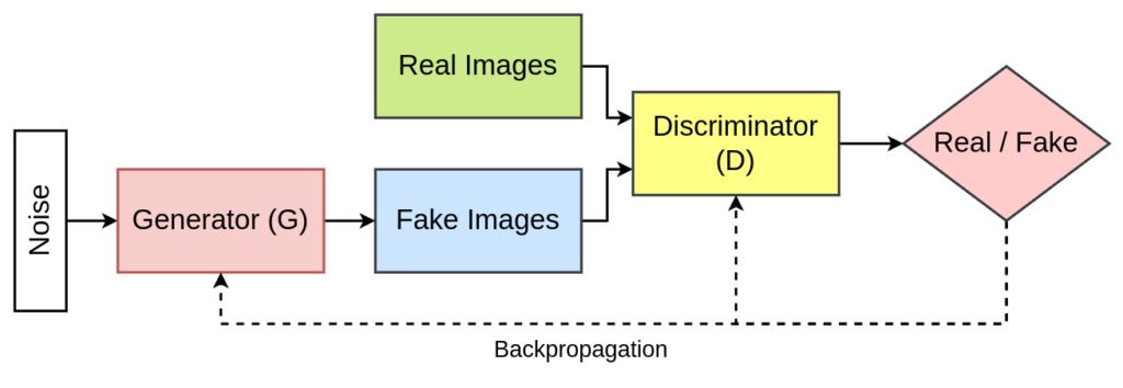
GAN stands for Generative Adversarial Network, a framework in which two neural networks, a generator and a discriminator, compete against each other to produce and evaluate realistic synthetic data.
- The generator is a crucial component of a Generative Adversarial Network (GAN), designed to create synthetic data that resembles real data. it takes in random noise or a low-dimensional input vector (often called a “latent vector” or “z”) as its input and produces synthetic data which is similar to the input data, but not identical.
- The discriminator is used to evaluate and distinguish between real and synthetic data. It takes as input either real data or synthetic data produced by the generator and produces a probability score that indicates the likelihood of the input data being real. For example, it might output a value close to 1 for real data and a value close to 0 for synthetic data.
The idea of GAN was introduced by Goodfellow and his team in their 2014 paper “Generative Adversarial Networks.” These networks can produce synthetic images that closely resemble authentic originals, both visually and perceptually.
Read More: What is Generative Adversarial Network?
Project Structure
├── gan.py
├── saved_model
│   ├── d_model.h5
│   └── g_model.h5
└── test.py
- gan.py – It contains the code for defining both the generator and discriminator neural network along with training the complete GAN.
- saved_model – It is the directory which is used to save the weight file for both the generator and discriminator neural network.
- test.py – This Python file used the trained generator neural network to generate synthetic anime faces.
Implementation of GAN in TensorFlow – gan.py
First, we have to import all the required libraries and the functions we need for the implementation of the generative adversarial network.
import os
import time
import numpy as np
import cv2
from glob import glob
from matplotlib import pyplot
from sklearn.utils import shuffle
import tensorflow as tf
from tensorflow.keras import layers as L
from tensorflow.keras.models import Model
from tensorflow.keras.optimizers import Adam
Next, we will define the height, width and number of channels in the real images. The generated images would also have the same dimensions.
IMG_H = 64
IMG_W = 64
IMG_C = 3  ## Change this to 1 for grayscale.
Now, we will define a function called create_dir. This function helps to create an empty directory.
def create_dir(path):
    if not os.path.exists(path):
        os.makedirs(path)
Next, we will write a function named load_image. This function takes an image path and provides preprocessed images used for training.
def load_image(image_path):
    img = tf.io.read_file(image_path)
    img = tf.io.decode_png(img)
    img = tf.cast(img, tf.float32)
    img = (img - 127.5) / 127.5
    return img
The above load_image function does the following:
- It first reads the image file from the image_path variable.
- Next, it decodes it as a png image file.
- After that, its datatype is changed to float32.
- Now, the image pixel values are normalized to the range of [-1, +1].
- We finally return the image.
After preprocessing the image, we will define a function called tf_dataset.
def tf_dataset(images_path, batch_size):
    ds = tf.data.Dataset.from_tensor_slices(images_path)
    ds = ds.shuffle(buffer_size=1000).map(load_image, num_parallel_calls=tf.data.experimental.AUTOTUNE)
    ds = ds.batch(batch_size).prefetch(buffer_size=tf.data.experimental.AUTOTUNE)
    return ds
In this function, we will establish the training pipeline. This includes operations such as batching, shuffling, and applying transformations to the preprocessed images to prepare them for training.
Now, we are going to define our generator neural network.
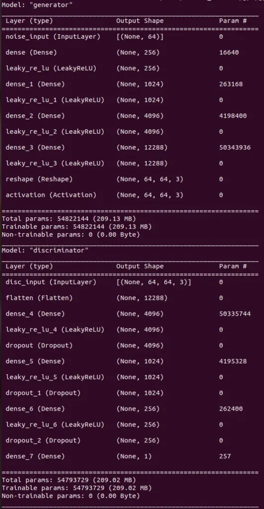
def build_generator(latent_dim):
    noise = L.Input((latent_dim), name="noise_input")

    ## 1.
    x = L.Dense(256)(noise)
    x = L.LeakyReLU(0.2)(x)

    ## 2.
    x = L.Dense(1024)(x)
    x = L.LeakyReLU(0.2)(x)

    ## 3.
    x = L.Dense(4096)(x)
    x = L.LeakyReLU(0.2)(x)

    ## 4.
    x = L.Dense(IMG_H * IMG_W * IMG_C)(x)
    x = L.LeakyReLU(0.2)(x)

    ## 5.
    x = L.Reshape((IMG_H, IMG_W, IMG_C))(x)

    fake_output = L.Activation("tanh")(x)

    return Model(noise, fake_output, name="generator")
Next, we will define the discriminator neural network.
def build_discriminator():
    inputs = L.Input((IMG_H, IMG_W, IMG_C), name="disc_input")

    ## 1.
    x = L.Flatten()(inputs)

    ## 2.
    x = L.Dense(4096)(x)
    x = L.LeakyReLU(0.2)(x)
    x = L.Dropout(0.3)(x)

    ## 3.
    x = L.Dense(1024)(x)
    x = L.LeakyReLU(0.2)(x)
    x = L.Dropout(0.3)(x)

    ## 4.
    x = L.Dense(256)(x)
    x = L.LeakyReLU(0.2)(x)
    x = L.Dropout(0.3)(x)

    ## 5.
    x = L.Dense(1)(x)

    return Model(inputs, x, name="discriminator")
After defining both the generator and discriminator, we will define a function called train_step. This function would help in training both the generator and discriminator neural network.
The function takes the following arguments:
- real_images – a batch of real images from the anime dataset.
- latent_dim – the size of the latent vector or noise, which is used as an input for the generator.
- generator – generator neural network.
- discriminator – discriminator neural network.
- g_opt – optimizer for generator neural network.
- d_opt – optimizer for discriminator neural network.
The function returns the discriminator loss and generator loss.
@tf.function
def train_step(real_images, latent_dim, generator, discriminator, g_opt, d_opt):
    batch_size = tf.shape(real_images)[0]
    bce_loss = tf.keras.losses.BinaryCrossentropy(from_logits=True, label_smoothing=0.1)

    ## Discriminator
    noise = tf.random.normal([batch_size, latent_dim])
    for _ in range(2):
        with tf.GradientTape() as dtape:
            generated_images = generator(noise, training=True)

            real_output = discriminator(real_images, training=True)
            fake_output = discriminator(generated_images, training=True)

            d_real_loss = bce_loss(tf.ones_like(real_output), real_output)
            d_fake_loss = bce_loss(tf.zeros_like(fake_output), fake_output)
            d_loss = d_real_loss + d_fake_loss

            d_grad = dtape.gradient(d_loss, discriminator.trainable_variables)
            d_opt.apply_gradients(zip(d_grad, discriminator.trainable_variables))

    with tf.GradientTape() as gtape:
        generated_images = generator(noise, training=True)
        fake_output = discriminator(generated_images, training=True)

        g_loss = bce_loss(tf.ones_like(fake_output), fake_output)

        g_grad = gtape.gradient(g_loss, generator.trainable_variables)
        g_opt.apply_gradients(zip(g_grad, generator.trainable_variables))

    return d_loss, g_loss
While training the GAN, we will also save a sample of synthetic images produced by the generator neural network. For that purpose, we will define a function called save_plot.
def save_plot(examples, epoch, n):
    n = int(n)
    examples = (examples + 1) / 2.0
    examples = examples * 255
    file_name = f"samples/generated_plot_epoch-{epoch+1}.png"

    cat_image = None
    for i in range(n):
        start_idx = i*n
        end_idx = (i+1)*n

        image_list = examples[start_idx:end_idx]
        if i == 0:
            cat_image = np.concatenate(image_list, axis=1)
        else:
            tmp = np.concatenate(image_list, axis=1)
            cat_image = np.concatenate([cat_image, tmp], axis=0)

    cv2.imwrite(file_name, cat_image)
Till now, we have defined all the functions and now we will work on the execution part of the program.
First, we will define some hyperparameters.
batch_size = 128
latent_dim = 64
num_epochs = 1000
n_samples = 100
After that, we will load all the images and create some empty directories.
images_path = glob("ML_DATASET/Anime Faces/*.png")
print(f"Images: {len(images_path)}")

create_dir("samples")
create_dir("saved_model")
The dataset can be downloaded from here: Anime Face Dataset.
Next, we will call both the generator and discriminator neural network, and then define their optimizer along with the learning rate.
g_model = build_generator(latent_dim)
d_model = build_discriminator()

g_model.summary()
d_model.summary()

d_optimizer = tf.keras.optimizers.Adam(learning_rate=0.0002, beta_1=0.5)
g_optimizer = tf.keras.optimizers.Adam(learning_rate=0.0002, beta_1=0.5)
Now, we will begin with the training part, by building the training pipeline using the tf_dataset function.
images_dataset = tf_dataset(images_path, batch_size)
seed = np.random.normal(size=(n_samples, latent_dim))
Here, seed refers to the initial latent vector which would be used during training to generate the synthetic images.
Now, we will have a for loop, inside which we have the code to train the GAN and then display their losses. We also save the weight file for both the generator and discriminator neural network along with the generated samples.
for epoch in range(num_epochs):
    start = time.time()

    d_loss = 0.0
    g_loss = 0.0
    for image_batch in images_dataset:
        d_batch_loss, g_batch_loss = train_step(image_batch, latent_dim, g_model, d_model, g_optimizer, d_optimizer)
        d_loss += d_batch_loss
        g_loss += g_batch_loss

    d_loss = d_loss/len(images_dataset)
    g_loss = g_loss/len(images_dataset)

    g_model.save("saved_model/g_model.h5")
    d_model.save("saved_model/d_model.h5")

    examples = g_model.predict(seed, verbose=0)
    save_plot(examples, epoch, np.sqrt(n_samples))

    time_taken = time.time() - start
    print(f"[{epoch+1:1.0f}/{num_epochs}] {time_taken:2.2f}s - d_loss: {d_loss:1.4f} - g_loss: {g_loss:1.4f}")
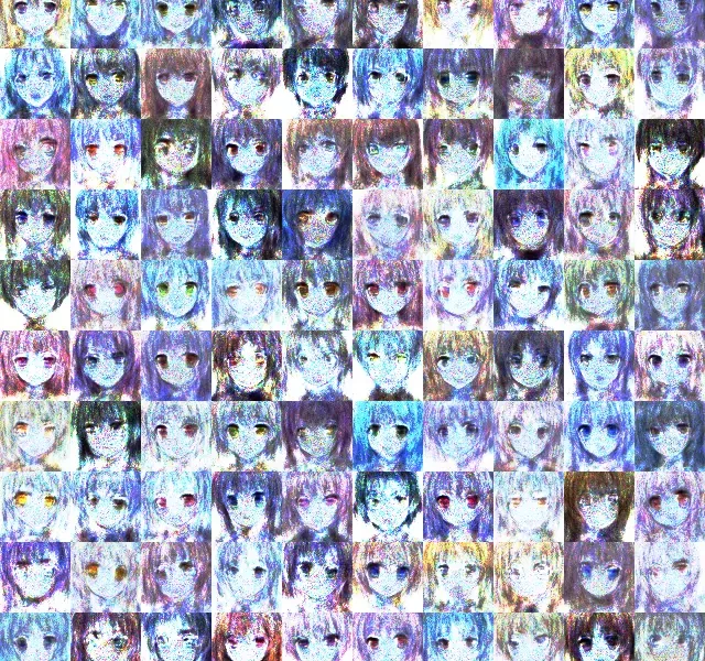
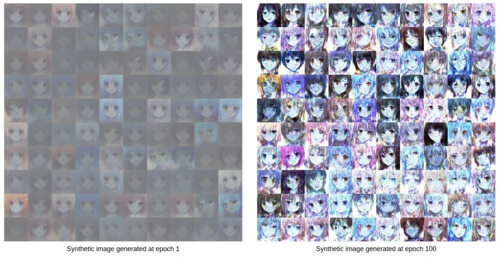
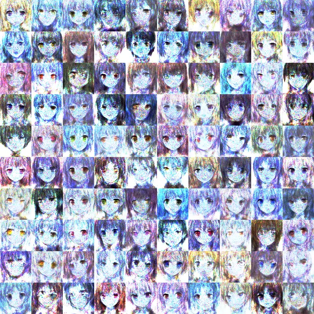
After the GAN is completely trained, the synthetic images generated during the training procedure show an improvement in performance.
Testing the Generator in GAN – test.py
Now, we will use the trained generator to generate some synthetic images which are similar to real images. So, first, we are going to import all the required libraries and functions.
import numpy as np
import cv2
from tensorflow.keras.models import load_model
from matplotlib import pyplot
Next again, we will define the same function called save_plot, which we have already defined in the gan.py file.
def save_plot(examples, n):
    n = int(n)
    examples = (examples + 1) / 2.0
    examples = examples * 255
    file_name = f"fake_sample.png"

    cat_image = None
    for i in range(n):
        start_idx = i*n
        end_idx = (i+1)*n

        image_list = examples[start_idx:end_idx]
        if i == 0:
            cat_image = np.concatenate(image_list, axis=1)
        else:
            tmp = np.concatenate(image_list, axis=1)
            cat_image = np.concatenate([cat_image, tmp], axis=0)

    cv2.imwrite(file_name, cat_image)
Now, let’s begin with the execution. First, we are going to load the generator model which we have trained.
model = load_model("saved_model/g_model.h5")
Now, we will have some have a latent vector from a normal distribution and then provide it to the generator model to generate some synthetic images.
n_samples = 100
latent_dim = 64
latent_points = np.random.normal(size=(n_samples, latent_dim))
examples = model.predict(latent_points)
save_plot(examples, np.sqrt(n_samples))
Conclusion
In this tutorial, we have learned about the basics of GAN (Generative Adversarial Network) and implemented a basic version of it in the TensorFlow framework. The performance of the vanilla GAN is not impressive. In future, we will work on more advanced versions of the GAN like DCGAN, which help in generating better synthetic or fake images.
To learn more about it, refer to the following
Do comment if you have any issues and follow me: