Conditional GAN in TensorFlow

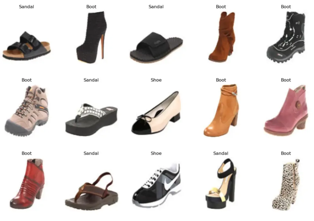
In this tutorial, we will implement the Conditional GAN (Generative Adversarial Network) in TensorFlow using Keras API. For this purpose, we will use the Shoe vs Sandal vs Boot Image dataset.

What is Conditional GAN

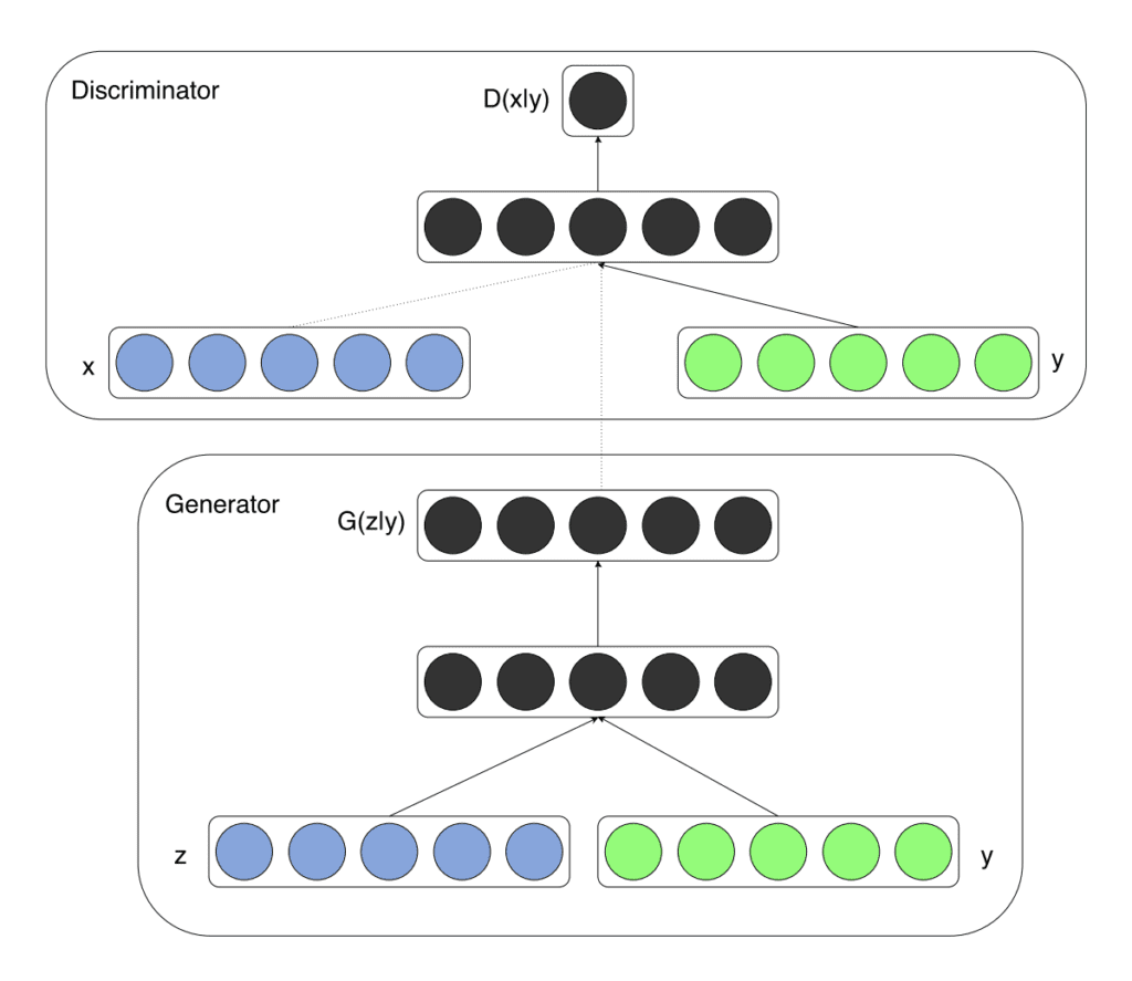
Conditional GAN, known as cGAN, is an extension of the traditional GAN framework introduced by Ian Goodfellow and his colleagues in 2014. While a standard GAN consists of a generator and a discriminator engaged in an adversarial training process to produce realistic data, a cGAN introduces a new element: conditioning. This means that the generator and the discriminator are given additional information, or context, guiding the generation process.

Read More: What is a Conditional GAN: Unleashing the Power of Context in Generative Models

Dataset

Now, we will move on to the implementation of the Conditional GAN on the Shoe vs Sandal vs Boot Image dataset. The dataset contains 15,000 RGB images of shoes, sandals and boots, 5000 images for each category. The images have a resolution of 136×102 pixels.

Project Structure

├── gan.py
├── saved_model
│   ├── d_model.h5
│   └── g_model.h5
└── test.py

• gan.py – It contains the code for defining both the generator and discriminator neural network along with training the complete GAN.

• saved_model – It is the directory which is used to save the weight file for both the generator and discriminator neural network.
• test.py – This Python file used the trained generator neural network to generate synthetic anime faces.

Implementation of GAN in TensorFlow – gan.py

First, we have to import all the required libraries and the functions we need for the implementation of the generative adversarial network.

import os
import time
import numpy as np
import cv2
from glob import glob
from matplotlib import pyplot
from sklearn.utils import shuffle
import tensorflow as tf
from tensorflow.keras import layers as L
from tensorflow.keras.models import Model
from tensorflow.keras.optimizers import Adam

Next, we will define the height, width and number of channels in the real images. The generated images would also have the same dimensions.

IMG_H = 96
IMG_W = 128
IMG_C = 3

Here, we have different height and width when compared with the original images. This is done to reduce the amount of GPU memory required to train the Conditional GAN, which helps to increase the batch size. In addition, it also reduces the training time each epoch.

Now, we will define a function called create_dir. This function helps to create an empty directory.

def create_dir(path):
    if not os.path.exists(path):
        os.makedirs(path)

Next, we will write a function named load_image. This function takes an image path and the label associated with the image.

The load_image function does the following:

1. It first reads the image file from the image_path variable.
2. Next, it decodes it as a png image file.
3. After that, its datatype is changed to float32.
4. Now, the image pixel values are normalized to the range of [-1, +1].
5. We finally return the image.

def load_image(image_path, label):
    img = tf.io.read_file(image_path)
    img = tf.io.decode_png(img)
    img = tf.image.resize(img, [IMG_H, IMG_W])
    img = tf.cast(img, tf.float32)
    img = (img - 127.5) / 127.5
    return img, label

In the above function, we have the following arguments:

1. image_path: The path to the image.
2. label: It is the integer value associated with a specific class.

The function returns a pre-processed image and an integer value representing a specific class label associated with the image.

After preprocessing the image, we will define a function called tf_dataset.

def tf_dataset(images_path, images_label, batch_size):
    ds = tf.data.Dataset.from_tensor_slices((images_path, images_label))
    ds = ds.shuffle(buffer_size=1000).map(load_image, num_parallel_calls=tf.data.experimental.AUTOTUNE)
    ds = ds.batch(batch_size).prefetch(buffer_size=tf.data.experimental.AUTOTUNE)
    return ds

In this function, we will establish the training pipeline. This includes operations such as batching, shuffling, and applying transformations to the preprocessed images to prepare them for training.

Now, we are going to define our generator neural network.

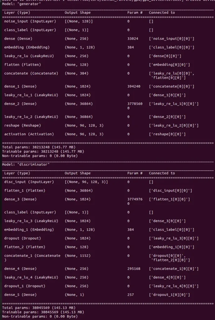
def build_generator(latent_dim, embed_dim, num_classes):
    noise = L.Input((latent_dim), name="noise_input")
    x = L.Dense(256)(noise)
    x = L.LeakyReLU(0.2)(x)

    label = L.Input((1), name="class_label")
    l = L.Embedding(num_classes, embed_dim)(label)
    l = L.Flatten()(l)

    x = L.Concatenate()([x, l])

    x = L.Dense(1024)(x)
    x = L.LeakyReLU(0.2)(x)

    x = L.Dense(IMG_H * IMG_W * IMG_C)(x)
    x = L.LeakyReLU(0.2)(x)

    x = L.Reshape((IMG_H, IMG_W, IMG_C))(x)
    fake_output = L.Activation("tanh")(x)

    return Model([noise, label], fake_output, name="generator")

In the build_generator function, the generator neural network takes the following three arguments as inputs:

1. latent_dim: It represents the size of the noise vector.
2. embed_dim: It represents the embedding dimensions. it is used to translate the class label, which is an integer value into a more useful representation.
3. num_class: Number of classes in the dataset.

The generator neural network uses the noise and class label as the input for the generator model and tries to generate data that is indistinguishable from real data of the specified class, effectively learning the underlying distribution.

Next, we will define the discriminator neural network.

def build_discriminator(embed_dim, num_classes):
    image = L.Input((IMG_H, IMG_W, IMG_C), name="disc_input")
    x = L.Flatten()(image)
    x = L.Dense(1024)(x)
    x = L.LeakyReLU(0.2)(x)
    x = L.Dropout(0.3)(x)

    label = L.Input((1), name="class_label")
    l = L.Embedding(num_classes, embed_dim)(label)
    l = L.Flatten()(l)

    x = L.Concatenate()([x, l])

    x = L.Dense(256)(x)
    x = L.LeakyReLU(0.2)(x)
    x = L.Dropout(0.3)(x)

    x = L.Dense(1)(x)

    return Model([image, label], x, name="discriminator")

The discriminator neural network also utilizes both the image (real or fake) and the class label. It tries to learn to discriminate between the real and the fake image produced by the generator neural network.

After defining both the generator and discriminator, we will define a function called train_step. This function would help in training both the generator and discriminator neural network.

@tf.function
def train_step(real_images, real_labels, latent_dim, num_classes, generator, discriminator, g_opt, d_opt):
    batch_size = tf.shape(real_images)[0]
    bce_loss = tf.keras.losses.BinaryCrossentropy(from_logits=True, label_smoothing=0.1)

    ## Discriminator
    noise = tf.random.normal([batch_size, latent_dim])

    for _ in range(3):
        with tf.GradientTape() as dtape:
            generated_images = generator([noise, real_labels], training=True)

            real_output = discriminator([real_images, real_labels], training=True)
            fake_output = discriminator([generated_images, real_labels], training=True)

            d_real_loss = bce_loss(tf.ones_like(real_output), real_output)
            d_fake_loss = bce_loss(tf.zeros_like(fake_output), fake_output)
            d_loss = d_real_loss + d_fake_loss

            d_grad = dtape.gradient(d_loss, discriminator.trainable_variables)
            d_opt.apply_gradients(zip(d_grad, discriminator.trainable_variables))

    with tf.GradientTape() as gtape:
        generated_images = generator([noise, real_labels], training=True)

        fake_output = discriminator([generated_images, real_labels], training=True)

        g_loss = bce_loss(tf.ones_like(fake_output), fake_output)

        g_grad = gtape.gradient(g_loss, generator.trainable_variables)
        g_opt.apply_gradients(zip(g_grad, generator.trainable_variables))

    return d_loss, g_loss

The function takes the following arguments:

1. real_images – a batch of real images from the anime dataset.
2. real_labels – a batch of class labels for the real_images.
3. latent_dim – the size of the latent vector or noise, which is used as an input for the generator.
4. num_classes – number of classes in the dataset.
5. generator – generator neural network.
6. discriminator – discriminator neural network.
7. g_opt – optimizer for generator neural network.
8. d_opt – optimizer for discriminator neural network.

The function returns the discriminator loss and generator loss.

While training the neural network, we train the discriminator neural network three times more than the generator neural network. This is done to strengthen the discriminator neural network, which further strengthens the generator neural network, and thus helps to produce more realistic synthetic images.

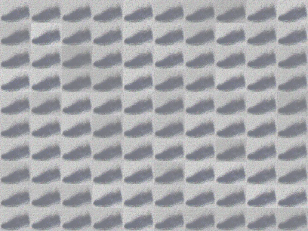
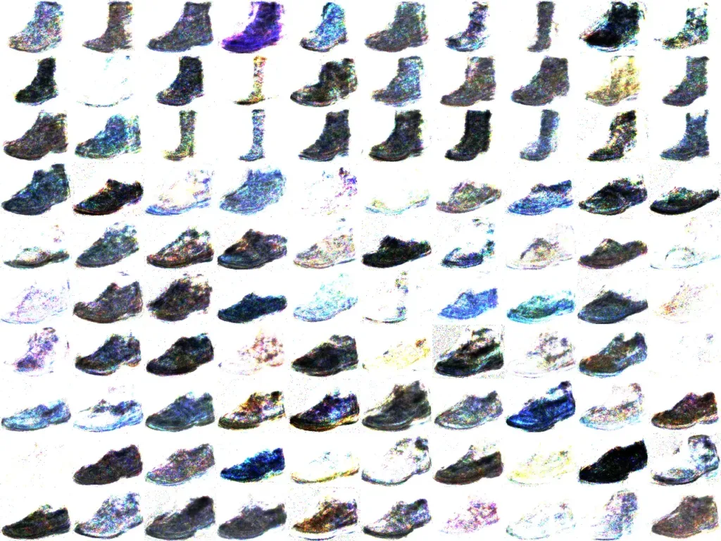
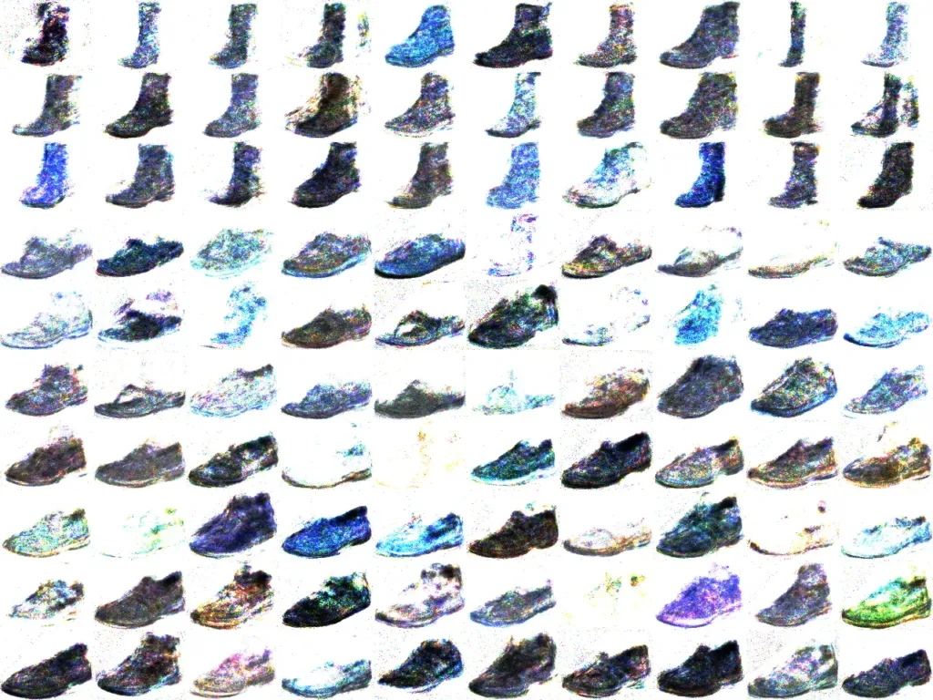
While training the GAN, we will also save a sample of synthetic images produced by the generator neural network. For that purpose, we will define a function called save_plot.

def save_plot(examples, epoch, n):
    n = int(n)
    examples = (examples + 1) / 2.0
    examples = examples * 255
    file_name = f"samples/generated_plot_epoch-{epoch+1}.png"

    cat_image = None
    for i in range(n):
        start_idx = i*n
        end_idx = (i+1)*n

        image_list = examples[start_idx:end_idx]
        if i == 0:
            cat_image = np.concatenate(image_list, axis=1)
        else:
            tmp = np.concatenate(image_list, axis=1)
            cat_image = np.concatenate([cat_image, tmp], axis=0)

    cv2.imwrite(file_name, cat_image)

Till now, we have defined all the functions and now we will work on the execution part of the program.

First, we will define some hyperparameters.

batch_size = 128
latent_dim = 128
embed_dim = 128
num_classes = 3
num_epochs = 1000
n_samples = 100
path = "../ML_DATASET/Shoe vs Sandal vs Boot Dataset"

After that, we will load all the images.

images_path = glob(f"{path}/*/*.jpg")

Next, we will work on the class label for the images.

labels_list = os.listdir(f"{path}")
print(f"Number of labels: {len(labels_list)}")
print(f"Labels: {labels_list}")

images_label = []
for path in images_path:
    name = path.split("/")[-2]
    index = labels_list.index(name)
    images_label.append(index)

print(f"Images: {len(images_path)} - Labels: {len(images_label)}")

Now, we will create some empty directories to save the model weights and the samples generated during training the Conditional GAN.

create_dir("samples")
create_dir("saved_model")

Next, we will call both the generator and discriminator neural network, and then define their optimizer along with the learning rate.

g_model = build_generator(latent_dim, embed_dim, num_classes)
d_model = build_discriminator(embed_dim, num_classes)

g_model.summary()
d_model.summary()

Now, we will begin with the training part, by defining the optimizer and building the training pipeline using the tf_dataset function.

d_optimizer = tf.keras.optimizers.Adam(learning_rate=0.0002, beta_1=0.5)
g_optimizer = tf.keras.optimizers.Adam(learning_rate=0.0002, beta_1=0.5)
images_dataset = tf_dataset(images_path, images_label, batch_size)

Now, we will define the seed and its associated class labels. Seed refers to the initial latent vector which would be used during training to generate the synthetic images.

seed = np.random.normal(size=(n_samples, latent_dim))
seed_class_label = [0, 0, 0, 1, 1, 1, 2, 2, 2, 2]
seed_label = []
for item in seed_class_label:
    seed_label += [item] * int(np.sqrt(n_samples))

seed_label = np.array(seed_label)

Now, we will have a for loop, inside which we have the code to train the GAN and then display their losses. We also save the weight file for both the generator and discriminator neural network along with the generated samples.

for epoch in range(num_epochs):
    start = time.time()

    d_loss = 0.0
    g_loss = 0.0
    for image_batch, label_batch in images_dataset:
        d_batch_loss, g_batch_loss = train_step(image_batch, label_batch, latent_dim, num_classes, g_model, d_model, g_optimizer, d_optimizer)
        d_loss += d_batch_loss
        g_loss += g_batch_loss

    d_loss = d_loss/len(images_dataset)
    g_loss = g_loss/len(images_dataset)

    g_model.save("saved_model/g_model.h5")
    d_model.save("saved_model/d_model.h5")

    examples = g_model.predict([seed, seed_label], verbose=0)
    save_plot(examples, epoch, np.sqrt(n_samples))

    time_taken = time.time() - start
    print(f"[{epoch+1:1.0f}/{num_epochs}] {time_taken:2.2f}s - d_loss: {d_loss:1.4f} - g_loss: {g_loss:1.4f}")

After the GAN is completely trained, the synthetic images generated during the training procedure show an improvement in performance.

Testing the Generator in GAN – test.py

Now, we will use the trained generator to generate some synthetic images which are similar to real images. So, first, we are going to import all the required libraries and functions.

import numpy as np
import cv2
from tensorflow.keras.models import load_model
from matplotlib import pyplot

Next again, we will define the same function called save_plot, which we have already defined in the gan.py file.

def save_plot(examples, n):
    n = int(n)
    examples = (examples + 1) / 2.0
    examples = examples * 255
    file_name = f"fake_sample.png"

    cat_image = None
    for i in range(n):
        start_idx = i*n
        end_idx = (i+1)*n

        image_list = examples[start_idx:end_idx]
        if i == 0:
            cat_image = np.concatenate(image_list, axis=1)
        else:
            tmp = np.concatenate(image_list, axis=1)
            cat_image = np.concatenate([cat_image, tmp], axis=0)

    cv2.imwrite(file_name, cat_image)

Now, we will begin with the execution and define some hyperparameters.

n_samples = 100
latent_dim = 128
embed_dim = 128
num_classes = 3

Next, we will load the weight file of the generator neural network.

model = load_model("saved_model/g_model.h5")

Now, we will define the seed and the labels for generating the required images.

latent_points = np.random.normal(size=(n_samples, latent_dim))

seed_class_label = [0, 0, 0, 1, 1, 1, 2, 2, 2, 2]
seed_label = []
for item in seed_class_label:
    seed_label += [item] * int(np.sqrt(n_samples))

seed_label = np.array(seed_label)

Now, we will provide the latent points (noise) and labels to the generative model and save the synthetic (fake) images.

examples = model.predict([latent_points, seed_label])
save_plot(examples, np.sqrt(n_samples))

Conclusion

In this tutorial, we have implemented a simple version of Conditional GAN in TensorFlow using Keras. The performance of the Conditional GAN is not impressive. In future, we will work on more advanced versions of the GAN like DCGAN, which help in generating better synthetic or fake images.

To learn more about it, refer to the following

• GAN – Google Advance Course
• How to Develop a Conditional GAN (cGAN) From Scratch
• Conditional GAN

Do comment if you have any issues and follow me:

• YouTube
• Facebook
• Twitter
• Instagram