In this tutorial, we are going to implement a Deep Convolutional Generative Adversarial Network (DCGAN) on Anime faces dataset. The code is written in TensorFlow 2.2 and Python3.8 .
According to Yann LeCun, the director of Facebook AI, GAN is the “most interesting idea in the last 10 years of machine learning.”
Overview:
- What are GANs
- How is DCGAN different from Vanilla GAN
- Anime Faces Dataset
- Implementation
- Summary
What is GAN
Generative Adversarial Network or GAN is a machine learning approach used for generative modelling designed by Ian Goodfellow and his colleagues in 2014. A GAN consists of two models: a generator and a discriminator, both of which are trained simultaneously by an adversarial process. The generator learns to generate images that look like real images, while the discriminator learns to differentiate between the real and the fake images.
We train both these models until the discriminator cannot differentiate between the real and the fake images.
Learn more: GAN – What is Generative Adversarial Network?
How is DCGAN different from Vanilla GAN
The vanilla GAN developed by Ian Goodfellow is based on the dense or fully-connected layer. The DCGAN or Deep Convolutional Generative Adversarial Network is an extension of the Generative Adversarial Network (GAN) and is built using the convolutional and transpose convolution layers. The DCGAN was first described in the paper Unsupervised Representation Learning With Deep Convolutional Generative Adversarial Networks by Radford et. al.
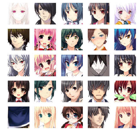
Anime Faces Dataset
The dataset consists of 21551 anime faces scraped from www.getchu.com, which are then cropped using the anime face detection algorithm. All images are resized to 64 * 64 for the sake of convenience.
Download: Anime Faces
Implementation
The following code demonstrates the implementation of Deep Convolutional Generative Adversarial Network (DCGAN) in TensorFlow on the Anime Faces dataset.
Import TensorFlow and Other Libraries
import os
import numpy as np
import cv2
from glob import glob
from matplotlib import pyplot
from sklearn.utils import shuffle
import tensorflow as tf
from tensorflow.keras.layers import *
from tensorflow.keras.models import Model
from tensorflow.keras.optimizers import Adam
Now, we define the dimensions of the anime images.
IMG_H = 64
IMG_W = 64
IMG_C = 3
The weight initialization for all the weights or kernels in the DCGAN must be randomlt initialized from a normal distribution with mean=0.0 and standard deviation = 0.02. This weights initializer is used in both the convolutional and the transpose convolutional layer.
w_init = tf.keras.initializers.RandomNormal(mean=0.0, stddev=0.02)
Loading and Preparing Dataset
The load_image function takes an image path and returns a tensor with values between -1 and 1. It does the following tasks:
- First, we read the image path.
- Next, we read the JPEG image file and return uint8 tensor.
- Next the image is resized with any extra cropping or padding required.
- The datatype of the image is changes to float 32.
- Now, we normalize the image pixel value between the range of -1 to 1.
def load_image(image_path):
    img = tf.io.read_file(image_path)
    img = tf.io.decode_jpeg(img)
    img = tf.image.resize_with_crop_or_pad(img, IMG_H, IMG_W)
    img = tf.cast(img, tf.float32)
    img = (img - 127.5) / 127.5
    return img
The tf_dataset function is used to set the TensorFlow dataset pipeline for the training.
def tf_dataset(images_path, batch_size):
    dataset = tf.data.Dataset.from_tensor_slices(images_path)
    dataset = dataset.shuffle(buffer_size=10240)
    dataset = dataset.map(load_image, num_parallel_calls=tf.data.experimental.AUTOTUNE)
    dataset = dataset.batch(batch_size)
    dataset = dataset.prefetch(buffer_size=tf.data.experimental.AUTOTUNE)
    return dataset
Transpose Convolution Blocks
The transpose convolution is used to build the generator model. It is used to increase the dimensions (height and width) of the incoming feature maps.
def deconv_block(inputs, num_filters, kernel_size, strides, bn=True):
    x = Conv2DTranspose(
        filters=num_filters,
        kernel_size=kernel_size,
        kernel_initializer=w_init,
        padding="same",
        strides=strides,
        use_bias=False
        )(inputs)

    if bn:
        x = BatchNormalization()(x)
        x = LeakyReLU(alpha=0.2)(x)
    return x
The strided-convolution is used to build the discriminator model.
def conv_block(inputs, num_filters, kernel_size, padding="same", strides=2, activation=True):
    x = Conv2D(
        filters=num_filters,
        kernel_size=kernel_size,
        kernel_initializer=w_init,
        padding=padding,
        strides=strides,
    )(inputs)

    if activation:
        x = LeakyReLU(alpha=0.2)(x)
        x = Dropout(0.3)(x)
    return x
Generator
The generator takes the random noise in the latent vector and map it to the data-space. As we are using RGB images, so our data-space means creating an RGB image.
The generator starts with a dense or fully-connected layer. After that it is followed the series of transpose convolution, batch normalization and the leaky relu activation function.
At the last, we use a convolution layer with three filters and tanh activation function to generate the RGB image.
def build_generator(latent_dim):
    f = [2**i for i in range(5)][::-1]
    filters = 32
    output_strides = 16
    h_output = IMG_H // output_strides
    w_output = IMG_W // output_strides

    noise = Input(shape=(latent_dim,), name="generator_noise_input")

    x = Dense(f[0] * filters * h_output * w_output, use_bias=False)(noise)
    x = BatchNormalization()(x)
    x = LeakyReLU(alpha=0.2)(x)
    x = Reshape((h_output, w_output, 16 * filters))(x)

    for i in range(1, 5):
        x = deconv_block(x,
            num_filters=f[i] * filters,
            kernel_size=5,
            strides=2,
            bn=True
        )

    x = conv_block(x,
        num_filters=3,
        kernel_size=5,
        strides=1,
        activation=False
    )
    fake_output = Activation("tanh")(x)

    return Model(noise, fake_output, name="generator")
Discriminator
The discriminator is a simple binary classification network that takes both the real and the fake image and outputs a probability of whether the given image is real or fake.
For this purpose, a series strided-convolution is used with leaky relu and the dropout with 0.3. At the last, we flatten the feature maps and use a fully-connected layer with one unit. Next, we apply a sigmoid activation function to the fully connected layer.
def build_discriminator():
    f = [2**i for i in range(4)]
    image_input = Input(shape=(IMG_H, IMG_W, IMG_C))
    x = image_input
    filters = 64
    output_strides = 16
    h_output = IMG_H // output_strides
    w_output = IMG_W // output_strides

    for i in range(0, 4):
        x = conv_block(x, num_filters=f[i] * filters, kernel_size=5, strides=2)

    x = Flatten()(x)
    x = Dense(1)(x)

    return Model(image_input, x, name="discriminator")
Complete DCGAN Model
The GAN class denotes the complete DCGAN model with the training step defined in it. It takes the discriminator model, generator mode and the loss function. The loss function used here is binary cross-entropy.
The train_step function is used for training the DCGAN model. The training starts with the discriminator. The discriminator is first trained on the fake images generated by the generator. After that it is trained on the real images from the anime faces dataset. Next, the generator is trained based on how well the discriminator is trained.
class GAN(Model):
    def __init__(self, discriminator, generator, latent_dim):
        super(GAN, self).__init__()
        self.discriminator = discriminator
        self.generator = generator
        self.latent_dim = latent_dim

    def compile(self, d_optimizer, g_optimizer, loss_fn):
        super(GAN, self).compile()
        self.d_optimizer = d_optimizer
        self.g_optimizer = g_optimizer
        self.loss_fn = loss_fn

    def train_step(self, real_images):
        batch_size = tf.shape(real_images)[0]

        for _ in range(2):
            ## Train the discriminator
            random_latent_vectors = tf.random.normal(shape=(batch_size, self.latent_dim))
            generated_images = self.generator(random_latent_vectors)
            generated_labels = tf.zeros((batch_size, 1))

            with tf.GradientTape() as ftape:
                predictions = self.discriminator(generated_images)
                d1_loss = self.loss_fn(generated_labels, predictions)
            grads = ftape.gradient(d1_loss, self.discriminator.trainable_weights)
            self.d_optimizer.apply_gradients(zip(grads, self.discriminator.trainable_weights))

            ## Train the discriminator
            labels = tf.ones((batch_size, 1))

            with tf.GradientTape() as rtape:
                predictions = self.discriminator(real_images)
                d2_loss = self.loss_fn(labels, predictions)
            grads = rtape.gradient(d2_loss, self.discriminator.trainable_weights)
            self.d_optimizer.apply_gradients(zip(grads, self.discriminator.trainable_weights))

        ## Train the generator
        random_latent_vectors = tf.random.normal(shape=(batch_size, self.latent_dim))
        misleading_labels = tf.ones((batch_size, 1))

        with tf.GradientTape() as gtape:
            predictions = self.discriminator(self.generator(random_latent_vectors))
            g_loss = self.loss_fn(misleading_labels, predictions)
        grads = gtape.gradient(g_loss, self.generator.trainable_weights)
        self.g_optimizer.apply_gradients(zip(grads, self.generator.trainable_weights))

        return {"d1_loss": d1_loss, "d2_loss": d2_loss, "g_loss": g_loss}
Saving image
def save_plot(examples, epoch, n):
    examples = (examples + 1) / 2.0
    for i in range(n * n):
        pyplot.subplot(n, n, i+1)
        pyplot.axis("off")
        pyplot.imshow(examples[i])
    filename = f"samples/generated_plot_epoch-{epoch+1}.png"
    pyplot.savefig(filename)
    pyplot.close()
Finally, running the code
if __name__ == "__main__":
    ## Hyperparameters
    batch_size = 128
    latent_dim = 128
    num_epochs = 60
    images_path = glob("data/*")

    d_model = build_discriminator()
    g_model = build_generator(latent_dim)

    # d_model.load_weights("saved_model/d_model.h5")
    # g_model.load_weights("saved_model/g_model.h5")

    d_model.summary()
    g_model.summary()

    gan = GAN(d_model, g_model, latent_dim)

    bce_loss_fn = tf.keras.losses.BinaryCrossentropy(from_logits=True, label_smoothing=0.1)
    d_optimizer = tf.keras.optimizers.Adam(learning_rate=0.0002, beta_1=0.5)
    g_optimizer = tf.keras.optimizers.Adam(learning_rate=0.0002, beta_1=0.5)
    gan.compile(d_optimizer, g_optimizer, bce_loss_fn)

    images_dataset = tf_dataset(images_path, batch_size)

    for epoch in range(num_epochs):
        gan.fit(images_dataset, epochs=1)
        g_model.save("saved_model/g_model.h5")
        d_model.save("saved_model/d_model.h5")

        n_samples = 25
        noise = np.random.normal(size=(n_samples, latent_dim))
        examples = g_model.predict(noise)
        save_plot(examples, epoch, int(np.sqrt(n_samples)))
Now, we are going to see the changes in the images generated at the first and the last epoch.
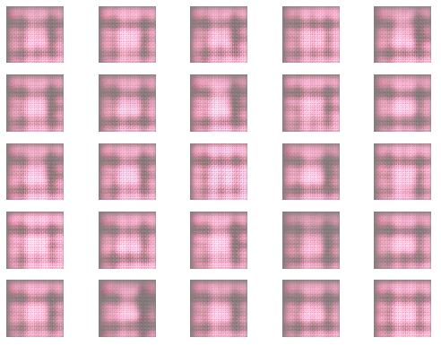

So, you can see after training the DCGAN on 60 epochs, the generator starts generating images that look real.
Summary
In this tutorial, we learn about implementing the Deep Convolutional Generative Adversarial Network (DCGAN) on the anime faces dataset. I hope after this tutorial, you will start building your own DCGANs.
Still have some questions, comment below and I will do my best to answer. For more updates. Follow me.
Further Reading
- Deep Convolutional Generative Adversarial Network by TensorFlow.
- DCGAN TUTORIAL by PyTorch.


Thanks for the tutorial. Why do you normalize the the data to [-1, 1]? I usually see (x – mean) / stddev used, but I’m guessing that’s not suitable for data like this…can you give some theory on the choice of normalization?
Cheers,
Steve
Which parts should be modified if we have inputs with higher heights and widths (128 x 128 or 256 x 256)? both Generator and discriminator?
Neither, there are global parameters IMG_W and IMG_H.
Thanks for the example of DCGAN, works well.
I have one question though. I see that there are dropout layers specified, however I think they do nothing unless in model call training=True is specified, since default is training=None.