Logistic Regression in TensorFlow

Logistic Regression is a popular machine-learning algorithm that is used for classification tasks. In this tutorial, we will learn how to implement Logistic Regression in TensorFlow 2.0 using the tf.keras.Model API. We will also learn how to split our data into training, validation, and testing sets in order to train and evaluate our model.

Related Post

• Implementing Linear Regression in TensorFlow

Importing Libraries

First, we need to import the necessary libraries. We will be using TensorFlow, Numpy, and Matplotlib.

import tensorflow as tf
import numpy as np
import matplotlib.pyplot as plt
from sklearn import datasets
from sklearn.model_selection import train_test_split

Loading the Data

Next, we will load our data. We will use the Iris dataset for this tutorial. The Iris dataset contains 150 samples of iris flowers, with 50 samples of each species (setosa, versicolor, and virginica). Each sample contains four features: sepal length, sepal width, petal length, and petal width. Our goal is to train a model that can classify the species of an iris flower based on these features.

iris = datasets.load_iris()
X = iris.data
y = iris.target

Splitting the Data

Before we can start training our model, we need to split our data into training, validation, and testing sets. We will use 80% of the data for training, 10% for validation, and 10% for testing.

X_train, X_test, y_train, y_test = train_test_split(X, y, test_size=0.2, random_state=42)
X_val, X_test, y_val, y_test = train_test_split(X_test, y_test, test_size=0.5, random_state=42)

Creating the Model

Now we can create our logistic regression model using the tf.keras.Model API. We will start by defining the input layer and the output layer. The input layer will have four neurons, one for each feature in the Iris dataset. The output layer will have three neurons, one for each species of iris.

class LogisticRegression(tf.keras.Model):
    def __init__(self):
        super(LogisticRegression, self).__init__()
        self.dense = tf.keras.layers.Dense(3, activation='softmax')

    def call(self, inputs):
        x = self.dense(inputs)
        return x

model = LogisticRegression()

Compiling the Model

Before we can start training our model, we need to compile it. We will use the Adam optimizer and the sparse categorical cross-entropy loss function.

model.compile(optimizer='adam', loss='sparse_categorical_crossentropy', metrics=['accuracy'])

Training the Model

Now we can train our model using the X_train and y_train data. We will train the model for 200 epochs and use the validation data (X_val, y_val) to evaluate the model during the training.

history = model.fit(X_train, y_train, epochs=200, validation_data=(X_val, y_val))

Evaluating the Model

Once our model is trained, we can use the test data (X_test, y_test) to evaluate its performance.

test_loss, test_acc = model.evaluate(X_test, y_test)
print('Test accuracy:', test_acc)

Output

1/1 [==============================] - 0s 23ms/step - loss: 0.6563 - accuracy: 0.8000
Test accuracy: 0.800000011920929

Plotting the Results

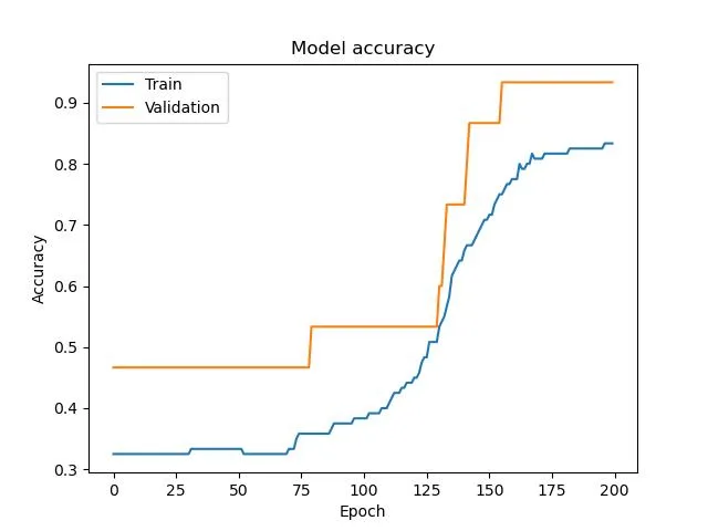
We can also plot the training and validation accuracy and loss to visualize the training process and check for overfitting.

plt.plot(history.history['accuracy'])
plt.plot(history.history['val_accuracy'])
plt.title('Model accuracy')
plt.ylabel('Accuracy')
plt.xlabel('Epoch')
plt.legend(['Train', 'Validation'], loc='upper left')
plt.savefig("acc.png")

plt.clf()
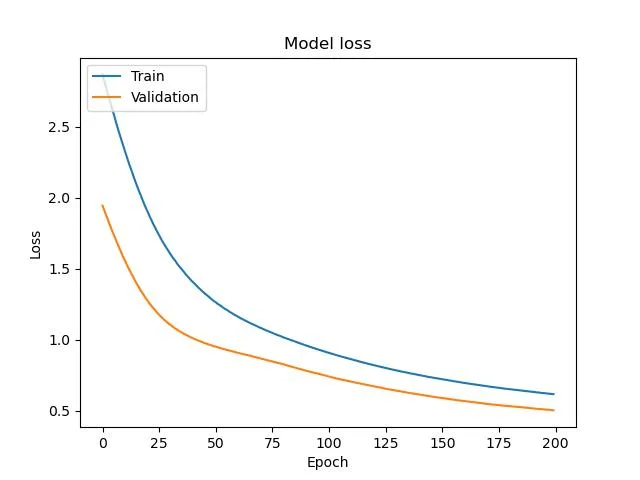
plt.plot(history.history['loss'])
plt.plot(history.history['val_loss'])
plt.title('Model loss')
plt.ylabel('Loss')
plt.xlabel('Epoch')
plt.legend(['Train', 'Validation'], loc='upper left')
plt.savefig("loss.png")

Conclusion

In this tutorial, we learned how to implement Logistic Regression in TensorFlow 2.0 using the tf.keras.Model API. We also learned how to split our data into training, validation, and testing sets in order to train and evaluate our model. We also learned how to plot the training and validation accuracy and loss in order to visualize the training process and check for overfitting. With this knowledge, you can now use Logistic Regression to tackle your own classification tasks in TensorFlow 2.0.

Still, have some questions or queries? Just comment below. For more updates. Follow me.

• YouTube
• Facebook
• Twitter
• Instagram